Panels

This page showcases panels implemented in iSEE and its known extensions.

Panels are grouped by package in which their are implemented (see the floating table of contents on the right).

Each panel is introduced by a brief description above a single screenshot that illustrates a representative output, and the code used to produce that particular panel output in a live app.

Note

Bear in mind that all those panel classes come with many options to alter their respective outputs. This gallery showcases only a fraction of what each of those panels can do. In all likelihood, if a panel seems to do almost what you have in mind, then there are options to make it do exactly that. Otherwise, options can be added, and more panel classes can be created; check out our resources to learn how!

iSEE

ColumnDataPlot

Visualise any combination of sample metadata stored in a SummarizedExperiment object.

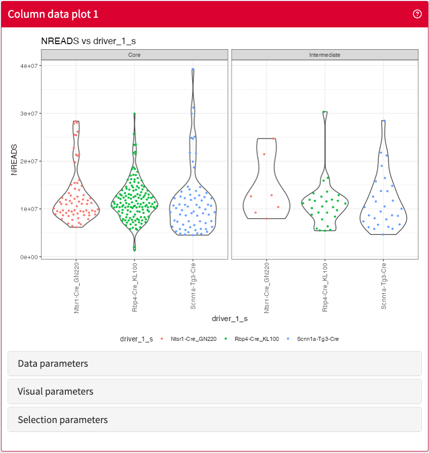
The ColumnDataPlot panel class.

Reproduce This Output

library(iSEE)
library(scRNAseq)
library(scater)

# Example data ----
sce <- ReprocessedAllenData(assays="tophat_counts")

sce <- logNormCounts(sce, exprs_values="tophat_counts")

# launch the app itself ----

app <- iSEE(sce, initial = list(
  ColumnDataPlot(
    PanelWidth = 8L,
    YAxis = "NREADS",
    XAxis = "Column data",
    XAxisColumnData = "driver_1_s",
    ColorBy = "Column data",
    ColorByColumnData = "driver_1_s",
    FacetColumnBy = "Column data",
    FacetColumnByColData = "Core.Type"
    )
))

if (interactive()) {
  shiny::runApp(app, port=1234)
}

ColumnDataTable

Browser and filter sample metadata stored in a SummarizedExperiment object.

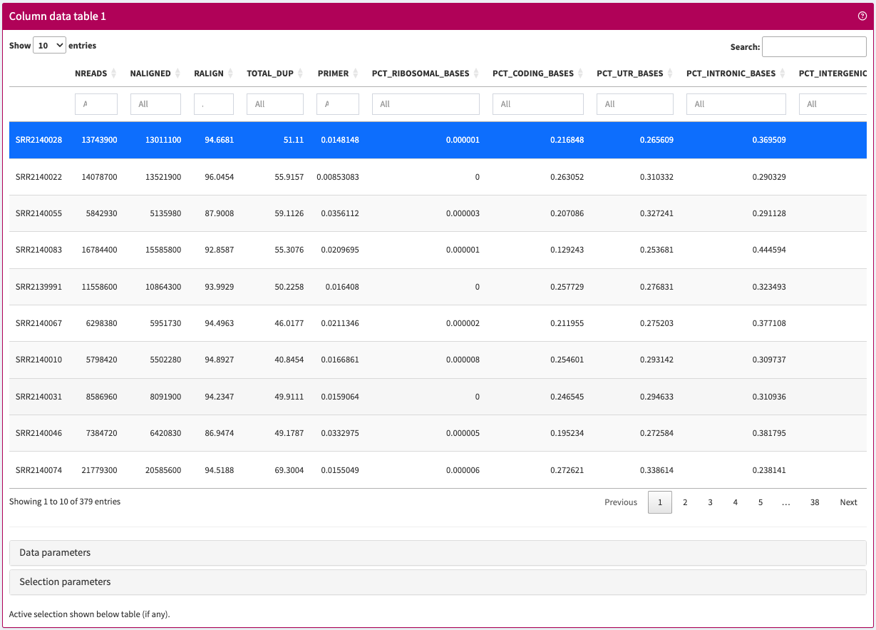
The ColumnDataTable panel class.

Reproduce This Output

library(iSEE)
library(scRNAseq)
library(scater)

# Example data ----
sce <- ReprocessedAllenData(assays="tophat_counts")

sce <- logNormCounts(sce, exprs_values="tophat_counts")

# launch the app itself ----

app <- iSEE(sce, initial = list(
  ColumnDataTable(
    PanelWidth = 12L
  )
))

if (interactive()) {
  shiny::runApp(app, port=1234)
}

ComplexHeatmapPlot

Visualise any number of features and samples in any assay stored in a SummarizedExperiment object.

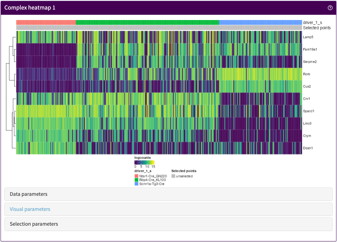
The ComplexHeatmapPlot panel class.

Reproduce This Output

library(iSEE)
library(scRNAseq)
library(scater)
library(tibble)
library(dplyr)

# Example data ----
sce <- ReprocessedAllenData(assays="tophat_counts")

sce <- logNormCounts(sce, exprs_values="tophat_counts")

rowData(sce)$ave_count <- rowMeans(assay(sce, "tophat_counts"))
rowData(sce)$n_cells <- rowSums(assay(sce, "tophat_counts") > 0)
rowData(sce)$row_var <- rowVars(assay(sce, "logcounts"))

# launch the app itself ----

# top 10 genes with highest variance in logcounts
gene_list <- c("Lamp5", "Fam19a1", "Cnr1", "Rorb", "Sparcl1", "Crym", "Lmo3",  "Serpine2", "Ddah1", "Cux2")

app <- iSEE(sce, initial = list(
  ComplexHeatmapPlot(
    PanelWidth = 12L,
    CustomRows = TRUE,
    CustomRowsText = paste0(paste0(gene_list, collapse = "\n"), "\n"),
    ColumnData = "driver_1_s",
    RowData = "row_var"
  )
))

if (interactive()) {
  shiny::runApp(app, port=1234)
}

FeatureAssayPlot

Visualise up to two features in any assay stored in a SummarizedExperiment object.

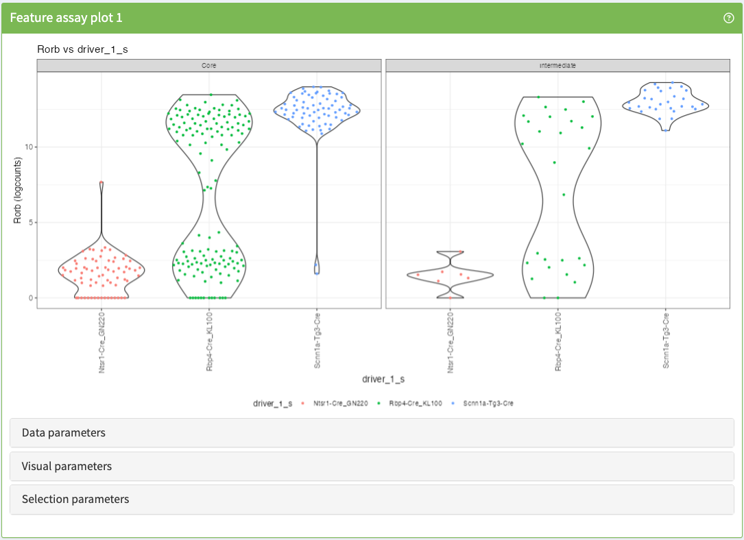
The FeatureAssayPlot panel class.

Reproduce This Output

library(iSEE)
library(scRNAseq)
library(scater)

# Example data ----
sce <- ReprocessedAllenData(assays="tophat_counts")

sce <- logNormCounts(sce, exprs_values="tophat_counts")

# launch the app itself ----

app <- iSEE(sce, initial = list(
  FeatureAssayPlot(
    PanelWidth = 12L,
    YAxisFeatureName = "Rorb",
    XAxis = "Column data", XAxisColumnData = "driver_1_s",
    ColorBy = "Column data", ColorByColumnData = "driver_1_s",
    FacetColumnBy = "Column data", FacetColumnByColData = "Core.Type"
  )
))

if (interactive()) {
  shiny::runApp(app, port=1234)
}

ReducedDimensionPlot

Visualise any two dimensions of any dimensionality reduction result stored in a SingleCellExperiment object.

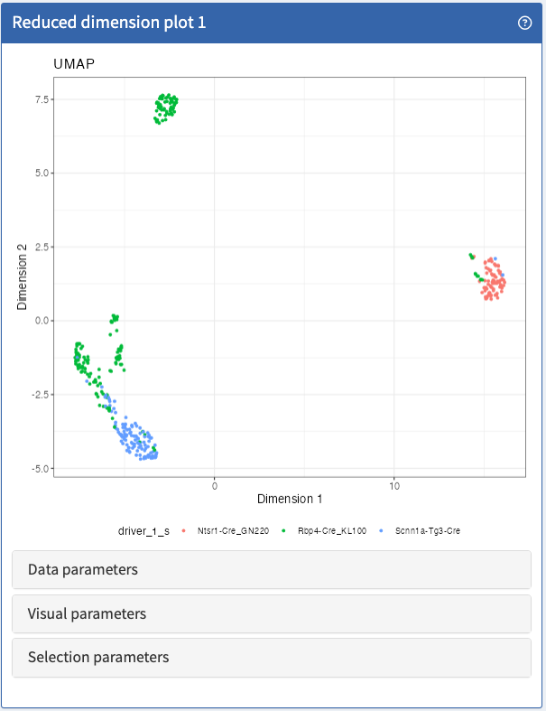
The ReducedDimensionPlot panel class.

Reproduce This Output

library(iSEE)
library(scRNAseq)
library(scater)

# Example data ----

sce <- ReprocessedAllenData(assays="tophat_counts")

sce <- logNormCounts(sce, exprs_values="tophat_counts")

sce <- runPCA(sce, ncomponents=4)
sce <- runUMAP(sce)

# launch the app itself ----

app <- iSEE(sce, initial = list(
  ReducedDimensionPlot(
    PanelWidth = 8L,
    Type = "UMAP",
    ColorBy = "Column data", ColorByColumnData = "driver_1_s")))

if (interactive()) {
  shiny::runApp(app, port=1234)
}

RowDataPlot

Visualise any combination of feature metadata stored in a SummarizedExperiment object.

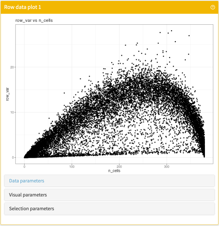
The RowDataPlot panel class.

Reproduce This Output

library(iSEE)
library(scRNAseq)
library(scater)

# Example data ----

sce <- ReprocessedAllenData(assays="tophat_counts")

sce <- logNormCounts(sce, exprs_values="tophat_counts")

rowData(sce)$row_var <- rowVars(assay(sce, "logcounts"))
rowData(sce)$n_cells <- rowSums(assay(sce, "logcounts") > 0)

# launch the app itself ----

app <- iSEE(sce, initial = list(
  RowDataPlot(
    PanelWidth = 12L,
    YAxis = "row_var",
    XAxis = "Row data",
    XAxisRowData = "n_cells"
  )
))

if (interactive()) {
  shiny::runApp(app, port=1234)
}

RowDataTable

Browse and filter feature metadata stored in a SummarizedExperiment object.

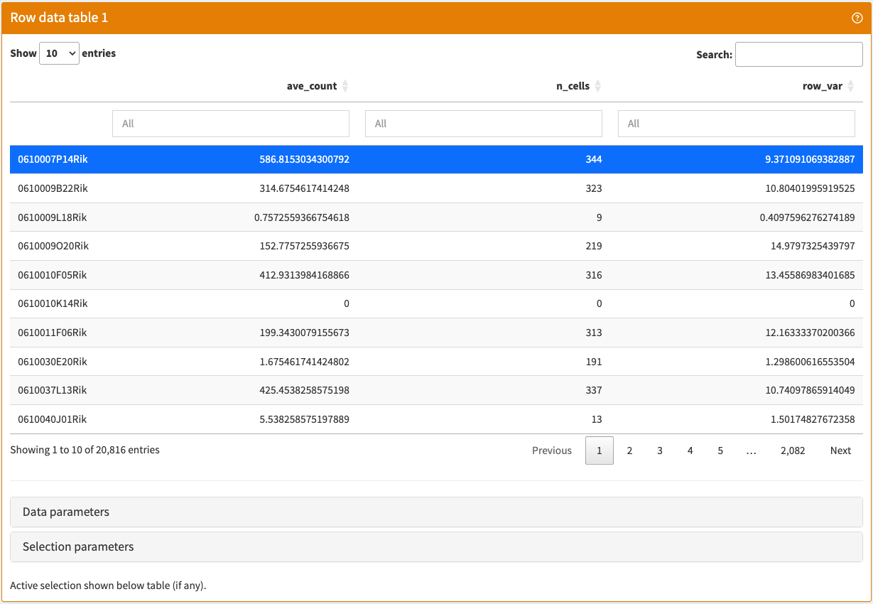
The RowDataTable panel class.

Reproduce This Output

library(iSEE)
library(scRNAseq)

# Example data ----

sce <- ReprocessedAllenData(assays="tophat_counts")

rowData(sce)$ave_count <- rowMeans(assay(sce, "tophat_counts"))
rowData(sce)$n_cells <- rowSums(assay(sce, "tophat_counts") > 0)

# launch the app itself ----

app <- iSEE(sce, initial = list(
  RowDataTable(
    PanelWidth = 12L
  )
))

if (interactive()) {
  shiny::runApp(app, port=1234)
}

SampleAssayPlot

Visualise up to two samples in any assay stored in a SummarizedExperiment object.

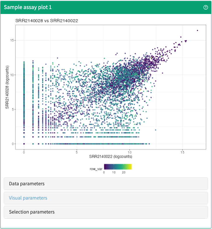
The SampleAssayPlot panel class.

Reproduce This Output

library(iSEE)
library(scRNAseq)
library(scater)

# Example data ----

sce <- ReprocessedAllenData(assays="tophat_counts")

sce <- logNormCounts(sce, exprs_values="tophat_counts")

rowData(sce)$row_var <- rowVars(assay(sce, "logcounts"))

# launch the app itself ----

app <- iSEE(sce, initial = list(
  SampleAssayPlot(
    PanelWidth = 12L,
    YAxisSampleName = "SRR2140028",
    XAxis = "Sample name", XAxisSampleName = "SRR2140022",
    ColorBy = "Row data", ColorByRowData = "row_var"
  )
))

if (interactive()) {
  shiny::runApp(app, port=1234)
}

iSEEde

DETable

Browse and filter any table of differential expression results embedded in a SummarizedExperiment object.

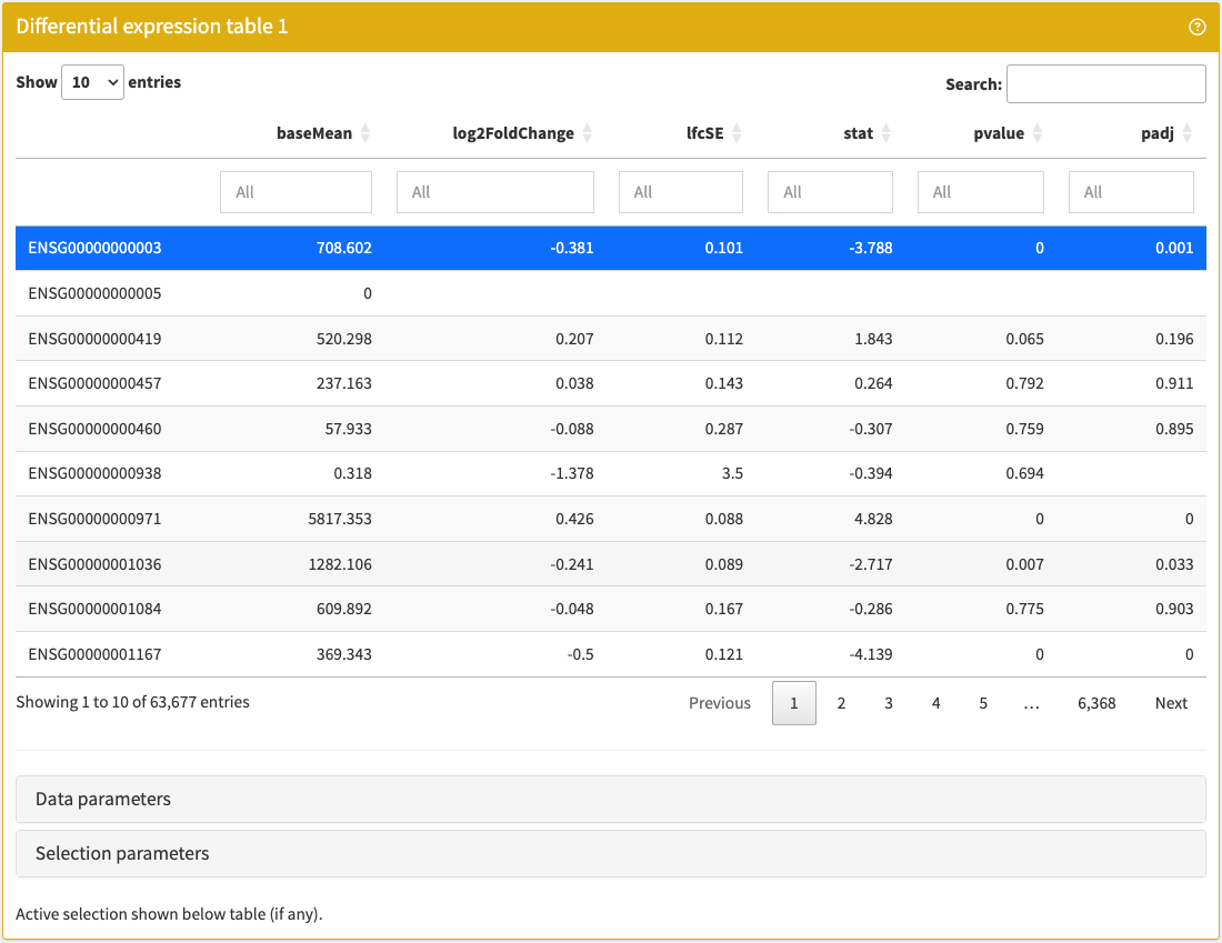
The DETable panel class.

Reproduce This Output

library(iSEE)
library(iSEEde)
library(airway)
library(DESeq2)

# Example data ----

data("airway")
airway$dex <- relevel(airway$dex, "untrt")

dds <- DESeqDataSet(airway, ~ 0 + dex + cell)

dds <- DESeq(dds)
res_deseq2 <- results(dds, contrast = list("dextrt", "dexuntrt"))

# iSEE / iSEEde ---

airway <- embedContrastResults(res_deseq2, airway, name = "dex: trt vs untrt")

app <- iSEE(airway, initial = list(
  DETable(
    PanelWidth = 12L,
    ContrastName="dex: trt vs untrt",
    RoundDigits = TRUE
  )
))

if (interactive()) {
  shiny::runApp(app)
}

LogFCLogFCPlot

Visualise the log-transformed fold-changes of any two differential expression contrasts embedded in a SummarizedExperiment object.

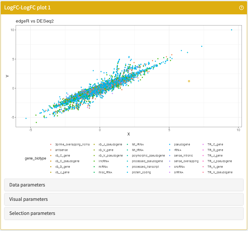
The LogFCLogFCPlot panel class.

Reproduce This Output

library("iSEEde")
library("airway")
library("edgeR")
library("DESeq2")
library("iSEE")

# Example data ----

data("airway")
airway$dex <- relevel(airway$dex, "untrt")

# DESeq2 ----

dds <- DESeqDataSet(airway, ~ 0 + dex + cell)

dds <- DESeq(dds)
res_deseq2 <- results(dds, contrast = list("dextrt", "dexuntrt"))

airway <- embedContrastResults(res_deseq2, airway, name = "DESeq2")

# edgeR ----

design <- model.matrix(~ 0 + dex + cell, data = colData(airway))

fit <- glmFit(airway, design, dispersion = 0.1)
lrt <- glmLRT(fit, contrast = c(-1, 1, 0, 0, 0))
res_edger <- topTags(lrt, n = Inf)

airway <- embedContrastResults(res_edger, airway, name = "edgeR")

# iSEE / iSEEde ---

airway <- registerAppOptions(airway, factor.maxlevels = 30, color.maxlevels = 30)

app <- iSEE(airway, initial = list(
  LogFCLogFCPlot(
    ContrastNameX = "DESeq2", ContrastNameY = "edgeR",
    ColorBy = "Row data",
    ColorByRowData = "gene_biotype",
    PanelWidth = 12L)
))

if (interactive()) {
  shiny::runApp(app)
}

MAPlot

Visualise the M and A values of any differential expression contrast embedded in a SummarizedExperiment object.

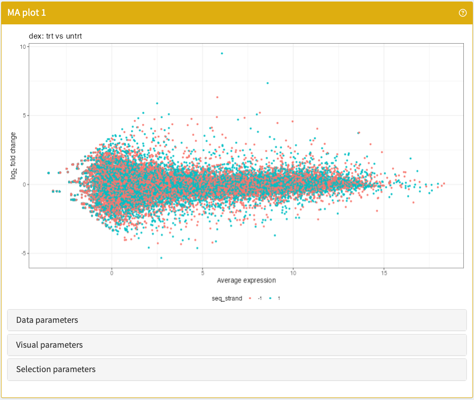
The MAPlot panel class.

Reproduce This Output

library("iSEEde")
library("airway")
library("DESeq2")
library("iSEE")

# Example data ----

data("airway")
airway$dex <- relevel(airway$dex, "untrt")
rowData(airway)$seq_strand <- factor(rowData(airway)$seq_strand)

dds <- DESeqDataSet(airway, ~ 0 + dex + cell)

dds <- DESeq(dds)
res_deseq2 <- results(dds, contrast = list("dextrt", "dexuntrt"))

# iSEE / iSEEde ---

airway <- embedContrastResults(res_deseq2, airway, name = "dex: trt vs untrt")

app <- iSEE(airway, initial = list(
  MAPlot(
    PanelWidth = 12L,
    ContrastName="dex: trt vs untrt",
    ColorBy = "Row data",
    ColorByRowData = "seq_strand"
  )
))

if (interactive()) {
  shiny::runApp(app)
}

VolcanoPlot

Visualise the P values and log-transformed fold-changes of any differential expression contrast embedded in a SummarizedExperiment object.

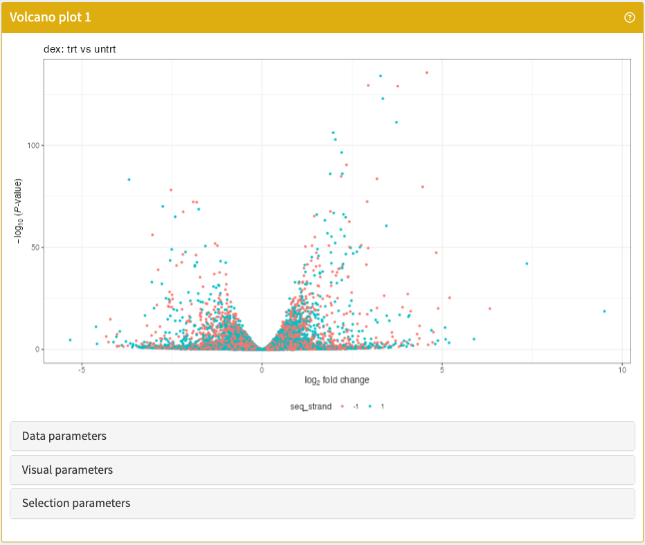
The VolcanoPlot panel class.

Reproduce This Output

library(iSEE)
library(iSEEde)
library(airway)
library(DESeq2)

# Example data ----

data("airway")
airway$dex <- relevel(airway$dex, "untrt")
rowData(airway)$seq_strand <- factor(rowData(airway)$seq_strand)

dds <- DESeqDataSet(airway, ~ 0 + dex + cell)

dds <- DESeq(dds)
res_deseq2 <- results(dds, contrast = list("dextrt", "dexuntrt"))

# iSEE / iSEEde ---

airway <- embedContrastResults(res_deseq2, airway, name = "dex: trt vs untrt")

app <- iSEE(airway, initial = list(
  VolcanoPlot(
    PanelWidth = 12L,
    ContrastName="dex: trt vs untrt",
    ColorBy = "Row data",
    ColorByRowData = "seq_strand"
  )
))

if (interactive()) {
  shiny::runApp(app)
}

iSEEhex

ReducedDimensionHexPlot

Same as ReducedDimensionPlot but summarised using hexagonal bins.

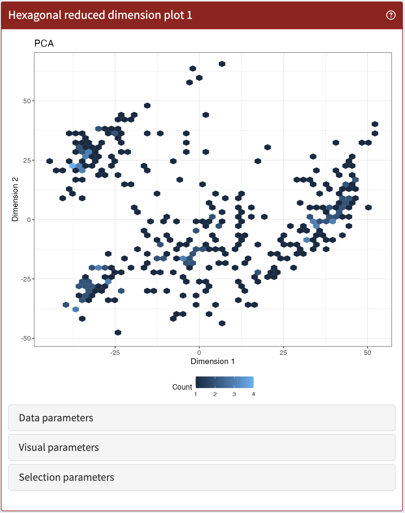
The ReducedDimensionHexPlot panel class.

Reproduce This Output

library(iSEE)
library(iSEEhex)
library(scRNAseq)
library(scater)

# Example data ----

sce <- ReprocessedAllenData(assays="tophat_counts")

sce <- logNormCounts(sce, exprs_values="tophat_counts")

sce <- runPCA(sce, ncomponents=4)

# launch the app itself ----

if (interactive()) {
  iSEE(sce, initial=list(
    ReducedDimensionHexPlot(PanelWidth = 12L, BinResolution=50)
  ))
}

iSEEpathways

FgseaEnrichmentPlot

GSEA enrichment plot produced by the fgsea package.

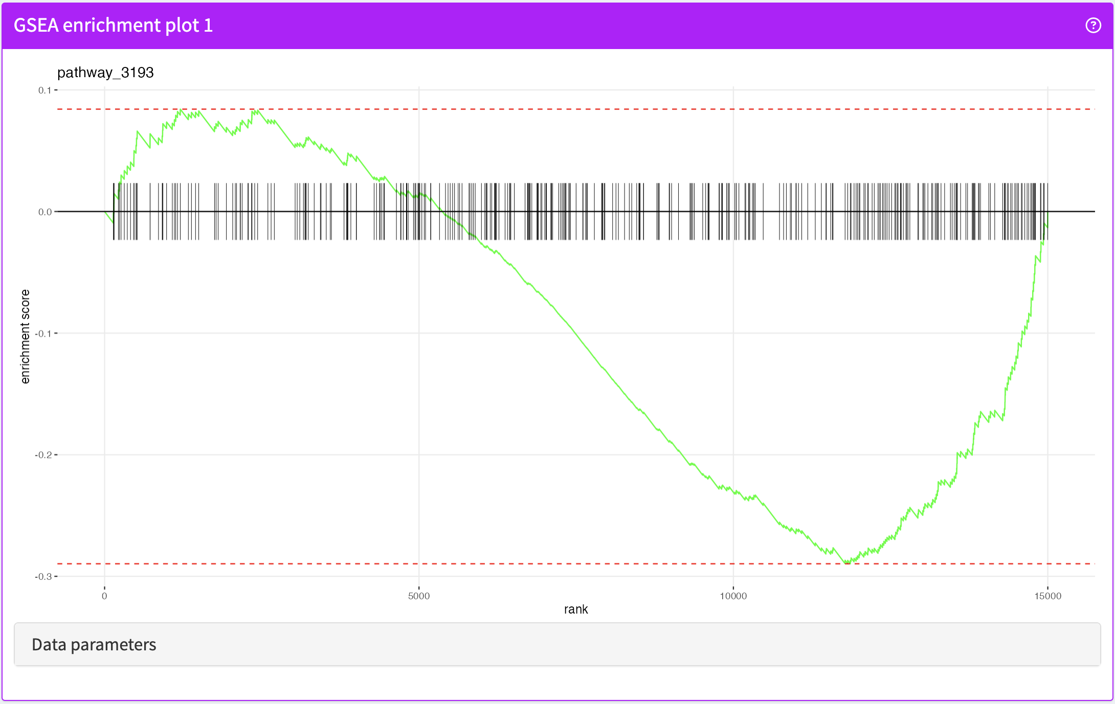
The FgseaEnrichmentPlot panel class.

Reproduce This Output

library(iSEE)
library(fgsea)
library(iSEEpathways)

# Example data ----

set.seed(1)
simulated_data <- simulateExampleData()

pathways_list <- simulated_data[["pathwaysList"]]
features_stat <- simulated_data[["featuresStat"]]
se <- simulated_data[["summarizedexperiment"]]

# fgsea ----

set.seed(42)
fgseaRes <- fgsea(pathways = pathways_list,
  stats    = features_stat,
  minSize  = 15,
  maxSize  = 500)
fgseaRes <- fgseaRes[order(pval), ]

# iSEE / iSEEpathways ---

se <- embedPathwaysResults(fgseaRes, se, name = "fgsea", class = "fgsea", pathwayType = "simulated",
  pathwaysList = pathways_list, featuresStats = features_stat)

app <- iSEE(se, initial = list(
  FgseaEnrichmentPlot(ResultName="fgsea", PathwayId = "pathway_1350", PanelWidth = 12L)
))

if (interactive()) {
  shiny::runApp(app)
}

PathwaysTable

Browse and filter any table of gene set analysis results embedded in a SummarizedExperiment object.

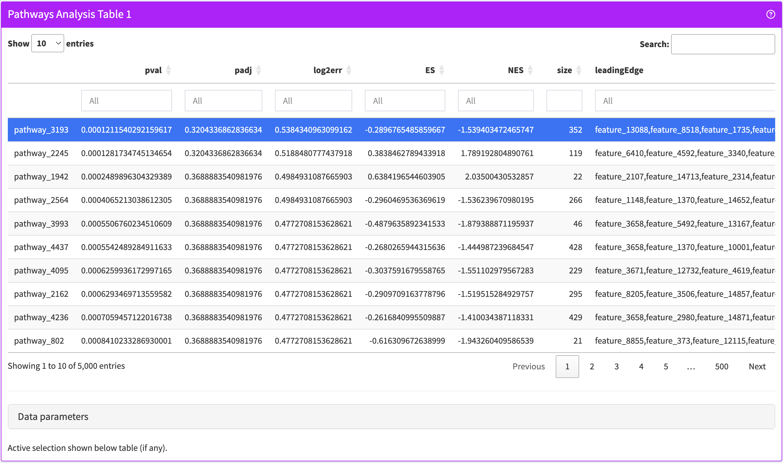
The PathwaysTable panel class.

Reproduce This Output

library(iSEE)
library(fgsea)
library(iSEEpathways)

# Example data ----

set.seed(1)
simulated_data <- simulateExampleData()

pathways_list <- simulated_data[["pathwaysList"]]
features_stat <- simulated_data[["featuresStat"]]
se <- simulated_data[["summarizedexperiment"]]

# fgsea ----

set.seed(42)
fgseaRes <- fgsea(pathways = pathways_list,
  stats    = features_stat,
  minSize  = 15,
  maxSize  = 500)
fgseaRes <- fgseaRes[order(pval), ]

# iSEE ---

se <- embedPathwaysResults(fgseaRes, se, name = "fgsea", class = "fgsea", pathwayType = "simulated",
  pathwaysList = pathways_list, featuresStats = features_stat)

app <- iSEE(se, initial = list(
  PathwaysTable(ResultName="fgsea", PanelWidth = 12L)
))

if (interactive()) {
  shiny::runApp(app)
}

iSEEu

AggregatedDotPlot

Represents groups of samples by dots, where colour scales with means assay value and size scales with proportion of non-zero values for selected features.

The AggregatedDotPlot panel class.

Reproduce This Output

library(iSEE)
library(scRNAseq)
library(scater)
library(iSEEu)

# Example data ----

sce <- ReprocessedAllenData(assays="tophat_counts")

sce <- logNormCounts(sce, exprs_values="tophat_counts")

# launch the app itself ----

if (interactive()) {
  iSEE(
    sce,
    initial = list(
      AggregatedDotPlot(
        ColumnDataLabel="Primary.Type",
        CustomRowsText = "Rorb\nSnap25\nFoxp2",
        # PanelHeight = 500L,
        PanelWidth = 12L
      )
    )
  )
}

DynamicMarkerTable

A table that dynamically identifies marker genes for a subset of samples transmitted from another panel. Comparisons are made between the active selection in the transmitting panel and either

• all non-selected points, if no saved selections are available, or
• each subset of points in each saved selection.

The DynamicMarkerTable panel class, alongside a ReducedDimensionPlot panel from which it receives a selection of samples.

Reproduce This Output

library(iSEE)
library(iSEEu)
library(scRNAseq)
library(scater)
library(scran)

sce <- ReprocessedAllenData(assays="tophat_counts")
sce <- logNormCounts(sce, exprs_values="tophat_counts")
sce <- runPCA(sce, ncomponents=4)

if (interactive()) {
  iSEE(sce, initial=list(
    ReducedDimensionPlot(
      PanelWidth=4L,
      BrushData = list(
        lasso = NULL, closed = TRUE,
        mapping = list(x = "X", y = "Y"),
        coord = structure(c(
          -47.8, -41.9, -14.6, -13.6, -19.1, -27.3, -33.6, -44, -47.8,
          -23.6, -44.1, -56.4, -46.9, -26.4, -17.4, -6.2, -5.4, -23.6),
          dim = c(9L, 2L))
        )
    ),
    DynamicMarkerTable(
      PanelWidth=8L,
      ColumnSelectionSource="ReducedDimensionPlot1"
    )
  ))
}

DynamicReducedDimensionPlot

A dimensionality reduction plot that dynamically recomputes the coordinates for the samples, based on a subset of samples and features transmitted from other panels.

The DynamicReducedDimensionPlot panel class, alongside a ReducedDimensionPlot panel from which it receives a selection of samples.

Reproduce This Output

library(iSEE)
library(iSEEu)
library(scRNAseq)
library(scater)

set.seed(1)
sce <- ReprocessedAllenData(assays="tophat_counts")
sce <- logNormCounts(sce, exprs_values="tophat_counts")
sce <- runPCA(sce, ncomponents=4)

if (interactive()) {
  iSEE(sce, initial=list(
    ReducedDimensionPlot(
      PanelWidth = 6L,
      BrushData = list(
        lasso = NULL, closed = TRUE,
        mapping = list(x = "X", y = "Y"),
        coord = structure(c(
          -47.8, -41.9, -14.6, -13.6, -19.1, -27.3, -33.6, -44, -47.8,
          -23.6, -44.1, -56.4, -46.9, -26.4, -17.4, -6.2, -5.4, -23.6),
          dim = c(9L, 2L))
      )
    ),
    DynamicReducedDimensionPlot(
      PanelWidth = 6L,
      Assay="logcounts",
      ColumnSelectionSource="ReducedDimensionPlot1"
    )
  ))
}

FeatureSetTable

A table where each row is itself a set of features (i.e., rows) and can be used to transmit such a feature set to another panel.

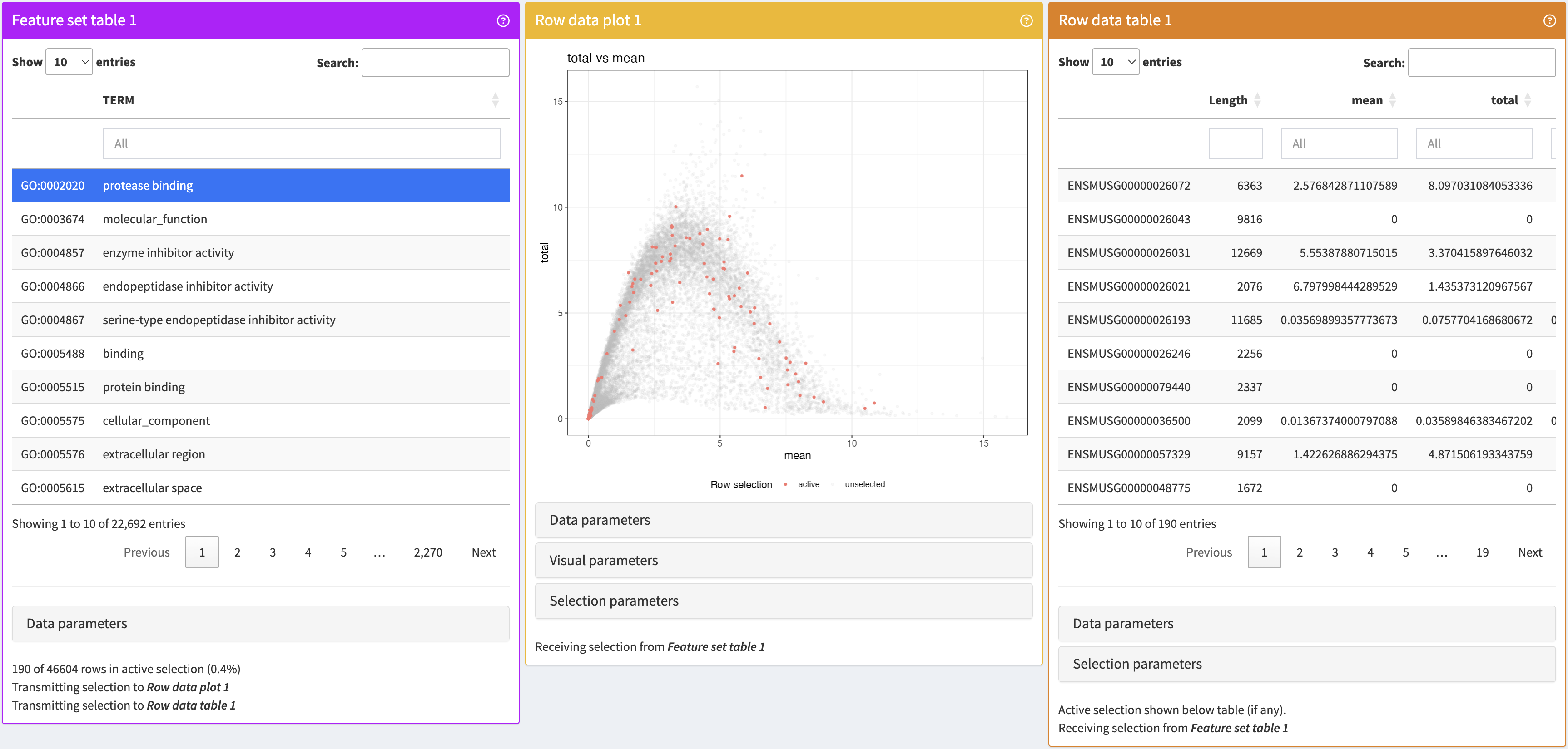
The FeatureSetTable panel class, alongside RowDataPlot and RowDataTable panels to which it transmits a feature set.

Reproduce This Output

library(iSEE)
library(iSEEu)
library(scRNAseq)
library(scater)
library(scran)
library(org.Mm.eg.db)

sce <- LunSpikeInData(location=FALSE)

sce <- logNormCounts(sce)

rowData(sce) <- cbind(rowData(sce), modelGeneVarWithSpikes(sce, "ERCC"))

cmds <- createGeneSetCommands(collections="GO",
  organism="org.Mm.eg.db", identifier="ENSEMBL")
sce <- registerFeatureSetCommands(sce, cmds)

# Setting up the application.

gst <- FeatureSetTable(
  Selected = "GO:0002020"
)

rdp <- RowDataPlot(
  YAxis="total",
  XAxis="Row data", XAxisRowData="mean",
  ColorBy="Row selection",
  RowSelectionSource="FeatureSetTable1"
)

rdt <- RowDataTable(
  RowSelectionSource="FeatureSetTable1"
)

if (interactive()) {
  iSEE(sce, initial=list(gst, rdp, rdt))
}

LogFCLogFCPlot

Precursor to the iSEEde::LogFCLogFCPlot class.

Warning

Deprecation imminent. Please use iSEEde::LogFCLogFCPlot() instead.

The LogFCLogFCPlot panel class.

Reproduce This Output

# Making up some results:
se <- SummarizedExperiment(matrix(rnorm(10000), 1000, 10))
rownames(se) <- paste0("GENE_", seq_len(nrow(se)))
rowData(se)$PValue1 <- runif(nrow(se))
rowData(se)$LogFC1 <- rnorm(nrow(se))
rowData(se)$PValue2 <- runif(nrow(se))
rowData(se)$LogFC2 <- rnorm(nrow(se))

if (interactive()) {
  iSEE(se, initial=list(
    LogFCLogFCPlot(
      PanelWidth = 12L,
      XAxisRowData="LogFC1", YAxis="LogFC2",
      XPValueField="PValue1", YPValueField="PValue2"
    )
  ))
}

MAPlot

Precursor to the iSEEde::MAPlot class.

Warning

Deprecation imminent. Please use iSEEde::MAPlot() instead.

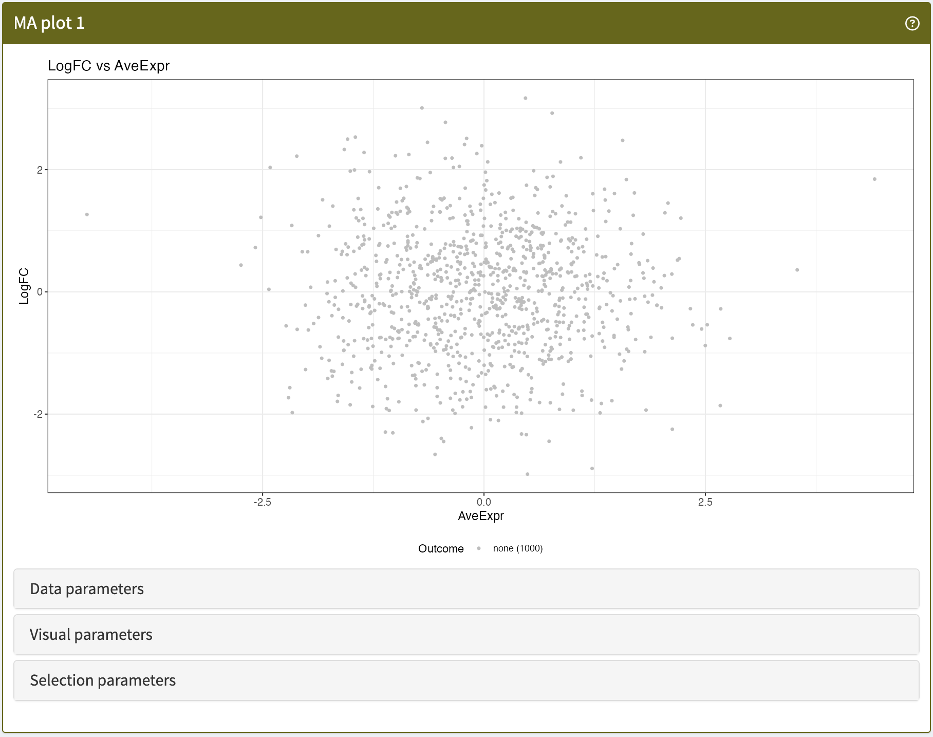
The MAPlot panel class.

Reproduce This Output

# Making up some results:
se <- SummarizedExperiment(matrix(rnorm(10000), 1000, 10))
rownames(se) <- paste0("GENE_", seq_len(nrow(se)))
rowData(se)$PValue <- runif(nrow(se))
rowData(se)$LogFC <- rnorm(nrow(se))
rowData(se)$AveExpr <- rnorm(nrow(se))

if (interactive()) {
  iSEE(se, initial=list(
    MAPlot(PanelWidth=12L)
  ))
}

MarkdownBoard

A panel providing an aceEditor that can be used to take notes within the app. Notes should be typed using Markdown syntax, and the panel continuously renders them in HTML format for preview.

The MarkdownBoard panel class.

Reproduce This Output

if (interactive()) {
  iSEE(SummarizedExperiment(), initial=list(
    MarkdownBoard(
      PanelWidth = 12L,
      Content = paste0(c(
        "# Level 1 header",
        "## Level 2 header",
        "**Bold** and *italic*.",
        "[Link](https://isee.github.io/)",
        "* Bullet point\n"),
        collapse = "\n\n"
      )
    )
  ))
}