Universe of iSEE panels
Kevin Rue-Albrecht
Kennedy Institute of Rheumatology, University of Oxford, Headington, Oxford OX3 7FY, UK.kevin.rue-albrecht@kennedy.ox.ac.uk
Federico Marini
Institute of Medical Biostatistics, Epidemiology and Informatics (IMBEI), MainzCenter for Thrombosis and Hemostasis (CTH), Mainzmarinif@uni-mainz.de
Charlotte Soneson
Friedrich Miescher Institute for Biomedical Research, BaselSIB Swiss Institute of Bioinformaticscharlottesoneson@gmail.com
Aaron Lun
infinite.monkeys.with.keyboards@gmail.com1 December 2025
Source:vignettes/iSEEu.Rmd
iSEEu.RmdOverview
The iSEE package
(Rue-Albrecht et al. 2018) provides a
general and flexible framework for interactively exploring
SummarizedExperiment objects. However, in many cases, more
specialized panels are required for effective visualization of specific
data types. The iSEEu
package implements a collection of such dedicated panel classes that
work directly in the iSEE application and can smoothly
interact with other panels. This allows users to quickly parametrize
bespoke apps for their data to address scientific questions of interest.
We first load in the package:
All the panels described in this document can be deployed by simply
passing them into the iSEE() function via the
initial= argument, as shown in the following examples.
Differential expression plots
To demonstrate the use of these panels, we will perform a
differential expression analysis on the airway
dataset with the edgeR
package. We store the resulting statistics in the rowData
of the SummarizedExperiment so that it can be accessed by
iSEE panels.
library(airway)
data(airway)

library(edgeR)
y <- DGEList(assay(airway), samples=colData(airway))
y <- y[filterByExpr(y, group=y$samples$dex),]
y <- calcNormFactors(y)

design <- model.matrix(~dex, y$samples)
y <- estimateDisp(y, design)
fit <- glmQLFit(y, design)
res <- glmQLFTest(fit, coef=2)

tab <- topTags(res, n=Inf)$table
rowData(airway) <- cbind(rowData(airway), tab[rownames(airway),])
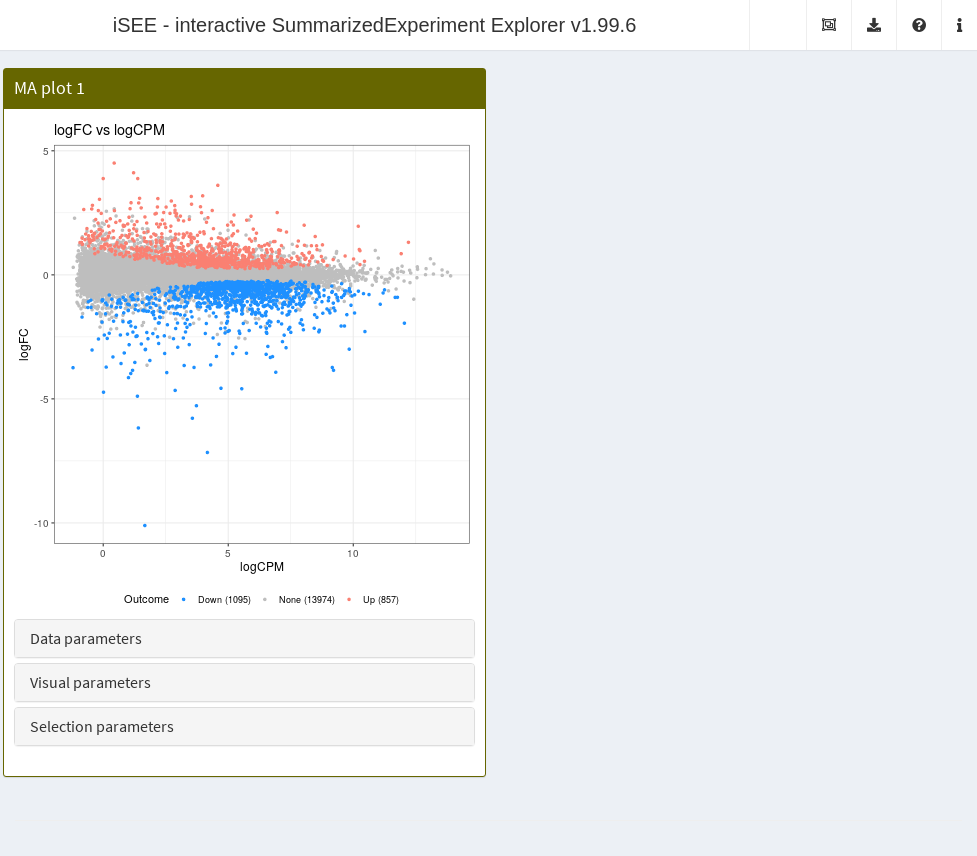
The MAPlot class creates a MA plot, i.e., with the
log-fold change on the y-axis and the average expression on the x-axis.
Features with significant differences in each direction are highlighted
and counted on the legend. Users can vary the significance threshold and
apply ad hoc filters on the log-fold change. This is a subclass
of the RowDataPlot so points can be transmitted to other
panels as multiple row selections. Instances of this class are created
like:
The VolcanoPlot class creates a volcano plot with the
log-fold change on the x-axis and the negative log-p-value on the
y-axis. Features with significant differences in each direction are
highlighted and counted on the legend. Users can vary the significance
threshold and apply ad hoc filters on the log-fold change. This
is a subclass of the RowDataPlot so points can be
transmitted to other panels as multiple row selections. Instances of
this class are created like:
vol.panel <- VolcanoPlot(PanelWidth=6L)
app <- iSEE(airway, initial=list(vol.panel))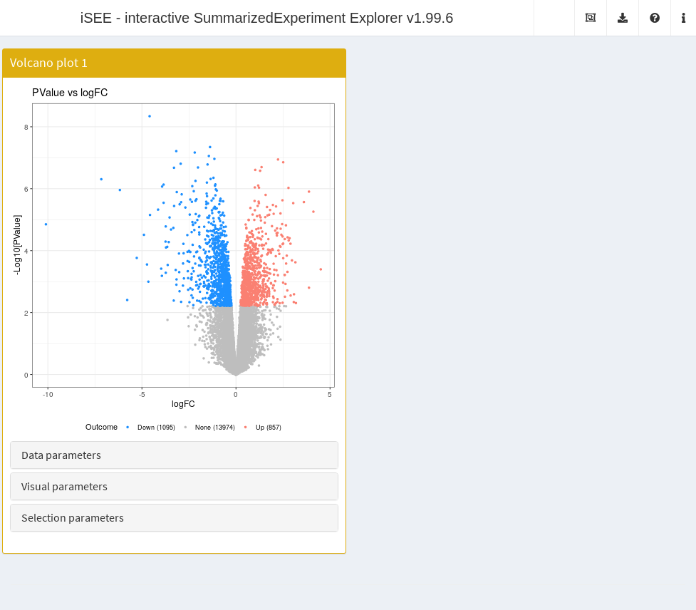
The LogFCLogFCPlot class creates a scatter plot of two
log-fold changes from different DE comparisons. This allows us to
compare DE results on the same dataset - or even from different
datasets, as long as the row names are shared. Users can vary the
significant threshold used to identify DE genes in either or both
comparisons. This is a subclass of the RowDataPlot so
points can be transmitted to other panels as multiple row selections.
Instances of this class are created like:
# Creating another comparison, this time by blocking on the cell line
design.alt <- model.matrix(~cell + dex, y$samples)
y.alt <- estimateDisp(y, design.alt)
fit.alt <- glmQLFit(y.alt, design.alt)
res.alt <- glmQLFTest(fit.alt, coef=2)

tab.alt <- topTags(res.alt, n=Inf)$table
rowData(airway) <- cbind(rowData(airway), alt=tab.alt[rownames(airway),])

lfc.panel <- LogFCLogFCPlot(PanelWidth=6L, YAxis="alt.logFC",
    YPValueField="alt.PValue")
app <- iSEE(airway, initial=list(lfc.panel))
Dynamically recalculated panels
To demonstrate, we will perform a quick analysis of a small dataset from the scRNAseq package. This involves computing normalized expression values and low-dimensional results using the scater package.
library(scRNAseq)
sce <- ReprocessedAllenData(assays="tophat_counts")

library(scater)
sce <- logNormCounts(sce, exprs_values="tophat_counts")
sce <- runPCA(sce, ncomponents=4)
sce <- runTSNE(sce)
The DynamicReducedDimensionPlot class creates a scatter
plot with a dimensionality reduction result, namely principal components
analysis (PCA),
-stochastic
neighbor embedding
(-SNE)
or uniform manifold and approximate projection (UMAP). It does so
dynamically on the subset of points that are selected in a transmitting
panel, allowing users to focus on finer structure when dealing with a
heterogeneous population. Calculations are performed using relevant
functions from the scater
package.
# Receives a selection from a reduced dimension plot.
dyn.panel <- DynamicReducedDimensionPlot(Type="UMAP", Assay="logcounts",
    ColumnSelectionSource="ReducedDimensionPlot1", PanelWidth=6L)

# NOTE: users do not have to manually create this, just
# copy it from the "Panel Settings" of an already open app.
red.panel <- ReducedDimensionPlot(PanelId=1L, PanelWidth=6L,
    BrushData = list(
        xmin = -45.943, xmax = -15.399, ymin = -58.560,
        ymax = 49.701, coords_css = list(xmin = 51.009,
            xmax = 165.009, ymin = 39.009,
            ymax = 422.009), coords_img = list(xmin = 66.313,
            xmax = 214.514, ymin = 50.712,
            ymax = 548.612), img_css_ratio = list(x = 1.300,
            y = 1.299), mapping = list(x = "X", y = "Y"),
        domain = list(left = -49.101, right = 57.228,
            bottom = -70.389, top = 53.519),
        range = list(left = 50.986, right = 566.922,
            bottom = 603.013, top = 33.155),
        log = list(x = NULL, y = NULL), direction = "xy",
        brushId = "ReducedDimensionPlot1_Brush",
        outputId = "ReducedDimensionPlot1"
    )
)

app <- iSEE(sce, initial=list(red.panel, dyn.panel))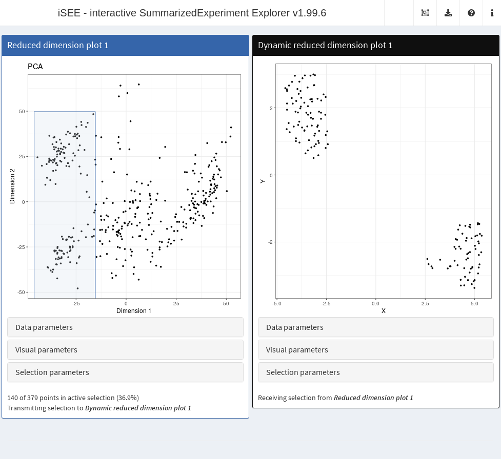
The DynamicMarkerTable class dynamically computes basic
differential statistics comparing assay values across groups of multiple
selections in a transmitting panel. If only the active selection exists
in the transmitting panel, a comparison is performed between the points
in that selection and all unselected points. If saved selections are
present, pairwise comparisons between the active selection and each
saved selection is performed and the results are combined into a single
table using the findMarkers() function from scran.
diff.panel <- DynamicMarkerTable(PanelWidth=8L, Assay="logcounts",
    ColumnSelectionSource="ReducedDimensionPlot1",)

# Recycling the reduced dimension panel above, adding a saved selection to
# compare to the active selection.
red.panel[["SelectionHistory"]] <- list(
    BrushData = list(
        xmin = 15.143, xmax = 57.228, ymin = -40.752,
        ymax = 25.674, coords_css = list(xmin = 279.009,
            xmax = 436.089, ymin = 124.009,
            ymax = 359.009), coords_img = list(xmin = 362.716,
            xmax = 566.922, ymin = 161.212,
            ymax = 466.712), img_css_ratio = list(x = 1.300,
            y = 1.299), mapping = list(x = "X", y = "Y"),
        domain = list(left = -49.101, right = 57.228,
            bottom = -70.389, top = 53.519),
        range = list(left = 50.986, right = 566.922,
            bottom = 603.013, top = 33.155),
        log = list(x = NULL, y = NULL), direction = "xy",
        brushId = "ReducedDimensionPlot1_Brush",
        outputId = "ReducedDimensionPlot1"
    )
)
red.panel[["PanelWidth"]] <- 4L # To fit onto one line.

app <- iSEE(sce, initial=list(red.panel, diff.panel))
Feature set table
The FeatureSetTable() class is a bit unusual in that its
rows do not correspond to any dimension of the
SummarizedExperiment. Rather, each row is a feature set
(e.g., from GO or KEGG) that, upon click, transmits a multiple row
selection to other panels. The multiple selection consists of all rows
in the chosen feature set, allowing users to identify the positions of
all genes in a pathway of interest on, say, a volcano plot. This is also
a rare example of a panel that only transmits and does not receive any
selections from other panels.
setFeatureSetCommands(createGeneSetCommands(identifier="ENSEMBL"))

gset.tab <- FeatureSetTable(Selected="GO:0002576",
    Search="platelet", PanelWidth=6L)

# This volcano plot will highlight the genes in the selected gene set.
vol.panel <- VolcanoPlot(RowSelectionSource="FeatureSetTable1",
    ColorBy="Row selection", PanelWidth=6L)

app <- iSEE(airway, initial=list(gset.tab, vol.panel))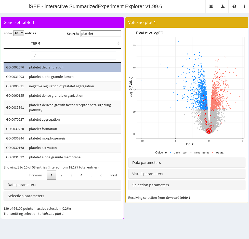
App modes
iSEEu
contains a number of “modes” that allow users to conveniently load an
iSEE instance in one of several common configurations:
-
modeEmpty()will launch an empty app, i.e., with no panels. This is occasionally useful to jump to the landing page where a user can then upload aSummarizedExperimentobject. -
modeGating()will launch an app with multiple feature assay panels that are linked to each other. This is useful for applying sequential restrictions on the data, equivalent to gating in a flow cytometry experiment. -
modeReducedDim()will launch an app with multiple reduced dimension plots. This is useful for examining different views of large high-dimensional datasets (e.g., single-cell studies).
Miscellaneous panels
iSEEu also includes a number of other panel types, that one can find useful within different contexts.
Coupled to each chunk of code listed below, it is possible to display a screenshot of the app showcasing them.
AggregatedDotPlot
app <- iSEE(
    sce,
    initial = list(
        AggregatedDotPlot(
            ColumnDataLabel="Primary.Type",
            CustomRowsText = "Rorb\nSnap25\nFoxp2",
            PanelHeight = 500L,
            PanelWidth = 8L
        )
    )
)

## To be later run as...
# app
## ... or
# shiny::runApp(app)
This can be very useful as an alternative to the
ComplexHeatmapPlot panel, as sometimes it is not just about
the shifts in average expression levels, but true biological signal can
be found e.g. in scenarios such as differential detection.
MarkdownBoard
The MarkdownBoard panel class renders Markdown notes,
user-supplied, into HTML to display inside the app.
app <- iSEE(
    sce,
    initial = list(
        MarkdownBoard(
            Content = "# `iSEE` notepad\n\nYou can enter anything here.\n\nA list of marker genes you might be interested into:\n\n- Snap25\n- Rorb\n- Foxp2\n\nThis makes it easier to copy-paste while staying inside `iSEE`.  \nAs you can notice, the full power of markdown is at your service.\n\nHave fun exploring your data, in an even more efficient manner!\n",
            PanelWidth = 8L,
            DataBoxOpen = TRUE
        )
    )
)

## To be later run as...
# app
## ... or
# shiny::runApp(app)
This is useful for displaying information alongside other panels, or for users to simply jot down their own notes (and re-use them more efficiently later).
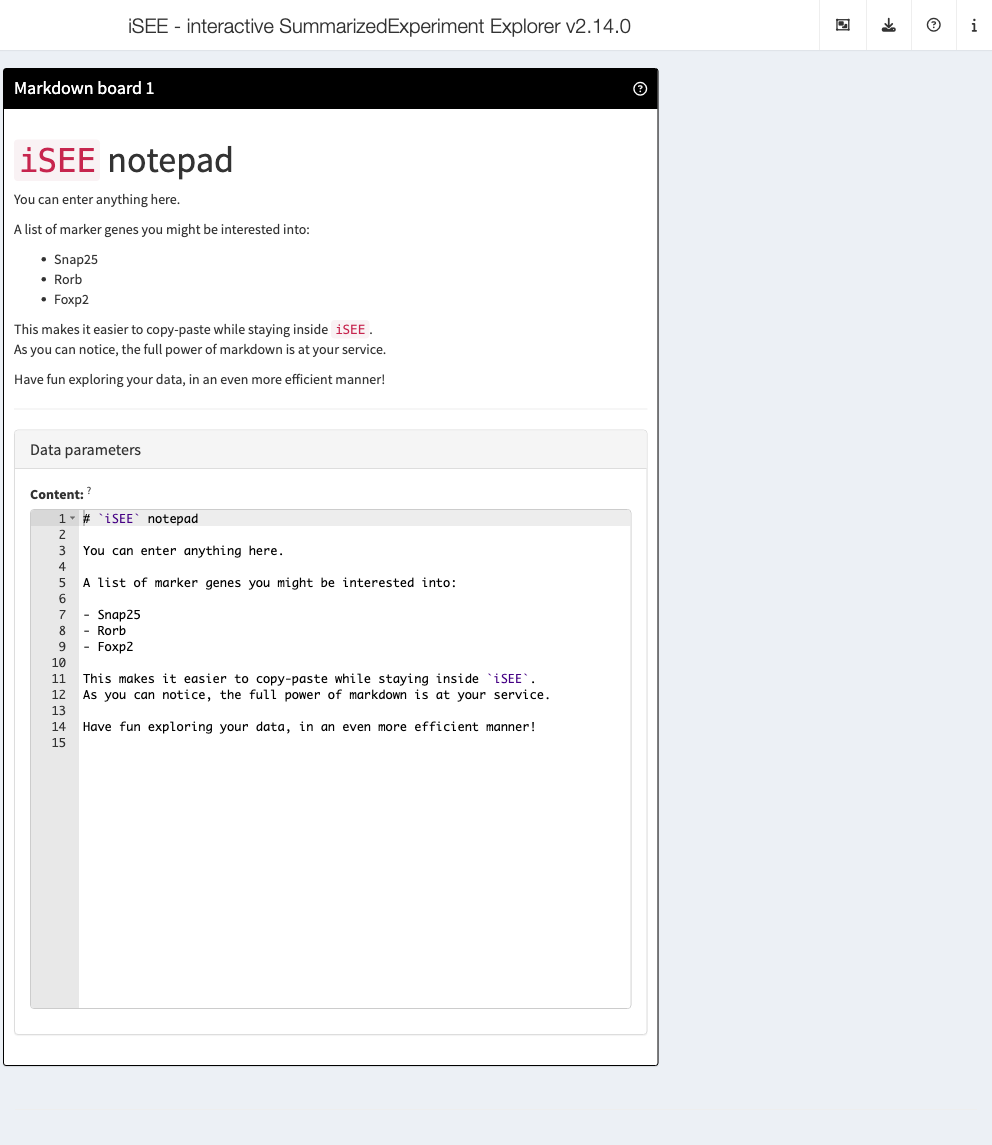
The content of the MarkdownBoard is included in the
Data parameters portion of the panel, as visible in the
screenshot.
iSEE will take care of rendering your notes into good-looking yet simple HTML, that can embedded in a variety of analytic workflows for the data under inspection.
Contributing to iSEEu
If you want to contribute to the development of the iSEEu package, here is a quick step-by-step guide:
- Fork the
iSEEurepository from GitHub (https://github.com/iSEE/iSEEu) and clone it locally.
git clone https://github.com/[your_github_username]/iSEEu.gitAdd the desired new files - start from the
Rfolder, then document viaroxygen2- and push to your fork. As an example you can check out to understand how things are supposed to work, there are several modes already defined in theR/directory. A typical contribution could include e.g. a function defining an iSEE mode, namedmodeXXX, whereXXXprovides a clear representation of the purpose of the mode. Please place each mode in a file of its own, with the same name as the function. The function should be documented (including an example), and any required packages should be added to theDESCRIPTIONfile.Once your
mode/function is done, consider adding some information in the package. Some examples might be a screenshot of the mode in action (to be placed in the folderinst/modes_img), and a well-documented example use case (maybe an entry in thevignettesfolder). Also add yourself as a contributor (ctb) to theDESCRIPTIONfile.Make a pull request to the original repo - the GitHub site offers a practical framework to do so, enabling comments, code reviews, and other goodies. The iSEE core team will evaluate the contribution and get back to you!
That’s pretty much it!
Using example data sets
Example data sets can often be obtained from an ExperimentHub package (e.g. from the scRNAseq package for single-cell RNA-sequencing data), and should not be added to the iSEEu package.
Documenting, testing, coding style and conventions
- If possible, please consider adding an example in the dedicated Roxygen preamble to show how to run each function
- If possible, consider adding one or more unit tests - we use the
testthatframework
We do follow some guidelines regarding the names given to variables, please abide to these for consistency with the rest of the codebase. Here are a few pointers:
- Keep the indentation as it is in the initial functions already available (4-spaces indentation).
- If writing text (e.g. in the vignette), please use one sentence per
line - this makes
git diffoperations easier to check. - When choosing variable names, try to keep the consistency with what
already is existing:
-
camelCasefor modes and other functions -
.function_namefor internals -
PanelClassNamefor panels -
.genericFunctionfor the API -
.scope1.scope2.namefor variable names in the cached info
-
If you intend to understand more in depth the internals of the iSEE framework, consider checking out the bookdown resource we put together at https://isee.github.io/iSEE-book/
Looking for constants within iSEE
Many of the “global” variables that are used in several places in iSEE are defined in the constants.R script in iSEE. We suggest to refer to those constants by their actual value rather than their internal variable name in downstream panel code. Both constant variable names and values may change at any time, but we will only announce changes to the constant value.
Session information
## R Under development (unstable) (2025-11-30 r89082)
## Platform: x86_64-pc-linux-gnu
## Running under: Ubuntu 24.04.3 LTS
##
## Matrix products: default
## BLAS:   /usr/lib/x86_64-linux-gnu/openblas-pthread/libblas.so.3
## LAPACK: /usr/lib/x86_64-linux-gnu/openblas-pthread/libopenblasp-r0.3.26.so;  LAPACK version 3.12.0
##
## locale:
##  [1] LC_CTYPE=en_US.UTF-8       LC_NUMERIC=C
##  [3] LC_TIME=en_US.UTF-8        LC_COLLATE=en_US.UTF-8
##  [5] LC_MONETARY=en_US.UTF-8    LC_MESSAGES=en_US.UTF-8
##  [7] LC_PAPER=en_US.UTF-8       LC_NAME=C
##  [9] LC_ADDRESS=C               LC_TELEPHONE=C
## [11] LC_MEASUREMENT=en_US.UTF-8 LC_IDENTIFICATION=C
##
## time zone: UTC
## tzcode source: system (glibc)
##
## attached base packages:
## [1] stats4    stats     graphics  grDevices utils     datasets  methods
## [8] base
##
## other attached packages:
##  [1] scater_1.39.0               ggplot2_4.0.1
##  [3] scuttle_1.21.0              scRNAseq_2.25.0
##  [5] edgeR_4.9.0                 limma_3.67.0
##  [7] airway_1.31.0               iSEEu_1.23.0
##  [9] iSEEhex_1.13.0              iSEE_2.23.1
## [11] SingleCellExperiment_1.33.0 SummarizedExperiment_1.41.0
## [13] Biobase_2.71.0              GenomicRanges_1.63.0
## [15] Seqinfo_1.1.0               IRanges_2.45.0
## [17] S4Vectors_0.49.0            BiocGenerics_0.57.0
## [19] generics_0.1.4              MatrixGenerics_1.23.0
## [21] matrixStats_1.5.0           BiocStyle_2.39.0
##
## loaded via a namespace (and not attached):
##   [1] splines_4.6.0            later_1.4.4              BiocIO_1.21.0
##   [4] bitops_1.0-9             filelock_1.0.3           tibble_3.3.0
##   [7] XML_3.99-0.20            lifecycle_1.0.4          httr2_1.2.1
##  [10] doParallel_1.0.17        lattice_0.22-7           ensembldb_2.35.0
##  [13] alabaster.base_1.11.1    magrittr_2.0.4           sass_0.4.10
##  [16] rmarkdown_2.30           jquerylib_0.1.4          yaml_2.3.11
##  [19] httpuv_1.6.16            otel_0.2.0               DBI_1.2.3
##  [22] RColorBrewer_1.1-3       abind_1.4-8              Rtsne_0.17
##  [25] AnnotationFilter_1.35.0  RCurl_1.98-1.17          rappdirs_0.3.3
##  [28] circlize_0.4.16          ggrepel_0.9.6            irlba_2.3.5.1
##  [31] alabaster.sce_1.11.0     pkgdown_2.2.0.9000       codetools_0.2-20
##  [34] DelayedArray_0.37.0      DT_0.34.0                tidyselect_1.2.1
##  [37] shape_1.4.6.1            UCSC.utils_1.7.0         farver_2.1.2
##  [40] viridis_0.6.5            ScaledMatrix_1.19.0      shinyWidgets_0.9.0
##  [43] BiocFileCache_3.1.0      GenomicAlignments_1.47.0 jsonlite_2.0.0
##  [46] BiocNeighbors_2.5.0      GetoptLong_1.1.0         iterators_1.0.14
##  [49] systemfonts_1.3.1        foreach_1.5.2            tools_4.6.0
##  [52] ragg_1.5.0               Rcpp_1.1.0               glue_1.8.0
##  [55] gridExtra_2.3            SparseArray_1.11.6       xfun_0.54
##  [58] mgcv_1.9-4               GenomeInfoDb_1.47.1      dplyr_1.1.4
##  [61] HDF5Array_1.39.0         gypsum_1.7.0             withr_3.0.2
##  [64] shinydashboard_0.7.3     BiocManager_1.30.27      fastmap_1.2.0
##  [67] rhdf5filters_1.23.1      shinyjs_2.1.0            rsvd_1.0.5
##  [70] digest_0.6.39            R6_2.6.1                 mime_0.13
##  [73] textshaping_1.0.4        colorspace_2.1-2         listviewer_4.0.0
##  [76] RSQLite_2.4.5            cigarillo_1.1.0          h5mread_1.3.1
##  [79] hexbin_1.28.5            rtracklayer_1.71.0       httr_1.4.7
##  [82] htmlwidgets_1.6.4        S4Arrays_1.11.1          pkgconfig_2.0.3
##  [85] gtable_0.3.6             blob_1.2.4               ComplexHeatmap_2.27.0
##  [88] S7_0.2.1                 XVector_0.51.0           htmltools_0.5.8.1
##  [91] bookdown_0.45            ProtGenerics_1.43.0      rintrojs_0.3.4
##  [94] clue_0.3-66              scales_1.4.0             alabaster.matrix_1.11.0
##  [97] png_0.1-8                knitr_1.50               rjson_0.2.23
## [100] nlme_3.1-168             curl_7.0.0               shinyAce_0.4.4
## [103] cachem_1.1.0             rhdf5_2.55.11            GlobalOptions_0.1.3
## [106] BiocVersion_3.23.1       parallel_4.6.0           miniUI_0.1.2
## [109] vipor_0.4.7              AnnotationDbi_1.73.0     restfulr_0.0.16
## [112] desc_1.4.3               pillar_1.11.1            grid_4.6.0
## [115] alabaster.schemas_1.11.0 vctrs_0.6.5              promises_1.5.0
## [118] BiocSingular_1.27.1      dbplyr_2.5.1             beachmat_2.27.0
## [121] xtable_1.8-4             cluster_2.1.8.1          beeswarm_0.4.0
## [124] evaluate_1.0.5           GenomicFeatures_1.63.1   cli_3.6.5
## [127] locfit_1.5-9.12          compiler_4.6.0           Rsamtools_2.27.0
## [130] rlang_1.1.6              crayon_1.5.3             ggbeeswarm_0.7.3
## [133] fs_1.6.6                 viridisLite_0.4.2        alabaster.se_1.11.0
## [136] BiocParallel_1.45.0      Biostrings_2.79.2        lazyeval_0.2.2
## [139] colourpicker_1.3.0       Matrix_1.7-4             ExperimentHub_3.1.0
## [142] bit64_4.6.0-1            Rhdf5lib_1.33.0          KEGGREST_1.51.1
## [145] statmod_1.5.1            shiny_1.11.1             alabaster.ranges_1.11.0
## [148] AnnotationHub_4.1.0      fontawesome_0.5.3        igraph_2.2.1
## [151] memoise_2.0.1            bslib_0.9.0              bit_4.6.0