Bonus content

Federico Marini¹, Kevin Rue-Albrecht², Charlotte Soneson³, Aaron Lun⁴, Najla Abassi⁵

Introduction

This vignette contains some additional examples of things that can be done using iSEE, going beyond the basic application interface.

iSEEde and iSEEpathways

iSEEde and iSEEpathways are ideal companion packages for exploring differential expression results in (e.g.) bulk RNA-seq data.

We will use the macrophage dataset (derived from the work of (Alasoo et al. 2018)), for which we have already run a differential expression analysis using DESeq2 (Love, Huber, and Anders 2014). The processed dataset is provided with the workshop package, and the processing code can be found in the accompanying script.

sce_macrophage <- readRDS(
  system.file("datasets", "sce_macrophage_readytouse.RDS",
              package = "iUSEiSEE")
)

library("iSEE")
library("iSEEde")
library("iSEEpathways")
library("AnnotationDbi")
library("org.Hs.eg.db")
#> 
library("GO.db")
#> 

iSEEde and iSEEpathways are two new Bioconductor packages that provide iSEE panels specifically aimed towards exploration of differential expression and pathway analysis results. More precisely, iSEEde provides the VolcanoPlot, MAPlot, LogFCLogFCPlot and DETable panels. These panels can be configured to extract data that was added via the embedContrastResults() function (see the processing script).

Let’s look at an example:

app <- iSEE(sce_macrophage, initial = list(
  iSEEde::DETable(
    ContrastName = "IFNgTRUE.SL1344TRUE.DESeq2",
    HiddenColumns = c("baseMean", "lfcSE", "stat")
  ),
  iSEEde::VolcanoPlot(ContrastName = "IFNgTRUE.SL1344TRUE.DESeq2"),
  iSEEde::MAPlot(ContrastName = "IFNgTRUE.SL1344TRUE.DESeq2")
))

Note how it is easy to switch to a different contrast in any of the panels.

app <- iSEE(sce_macrophage, initial = list(
  iSEEde::DETable(
    ContrastName = "IFNgTRUE.SL1344TRUE.DESeq2",
    HiddenColumns = c("baseMean", "lfcSE", "stat")
  ),
  iSEEde::VolcanoPlot(ContrastName = "IFNgTRUE.SL1344TRUE.DESeq2"),
  iSEEde::MAPlot(ContrastName = "IFNgTRUE.SL1344TRUE.DESeq2"),
  PathwaysTable(
    ResultName = "IFNgTRUE.SL1344TRUE.limma.fgsea",
    Selected = "GO:0046324"
  ),
  ComplexHeatmapPlot(
    RowSelectionSource = "PathwaysTable1",
    CustomRows = FALSE, ColumnData = "condition_name",
    ClusterRows = TRUE, Assay = "vst"
  ),
  FgseaEnrichmentPlot(
    ResultName = "IFNgTRUE.SL1344TRUE.limma.fgsea",
    PathwayId = "GO:0046324"
  )
))

iSEEfier

Let’s say we are interested in visualizing the expression of a list of specific marker genes in one view, or maybe we created different initial states separately, but would like to visualize them in the same instance. As we previously learned, we can do a lot of these tasks by launching the default interface with iSEE(sce), and adding/removing panels as desired. This can involve multiple manual steps (selecting the gene of interest, color by a specific colData column, …), or the execution of multiple lines of setup code. The iSEEfier package streamlines the process of starting (or if you will, firing up) an iSEE instance with a small chunk of code, avoiding the tedious way of setting up every iSEE panel individually.

In this section, we will illustrate a simple example of how to use iSEEfier. We will use the same pbmc3k data we worked with during this workshop.

We start by loading the data:

library("iSEEfier")

# import data
sce <- readRDS(
  file = system.file("datasets", "sce_pbmc3k.RDS", package = "iUSEiSEE")
)

sce
#> class: SingleCellExperiment 
#> dim: 32738 2643 
#> metadata(0):
#> assays(2): counts logcounts
#> rownames(32738): MIR1302-10 FAM138A ... AC002321.2 AC002321.1
#> rowData names(19): ENSEMBL_ID Symbol_TENx ... FDR_cluster11
#>   FDR_cluster12
#> colnames(2643): Cell1 Cell2 ... Cell2699 Cell2700
#> colData names(24): Sample Barcode ... labels_ont cell_ontology_labels
#> reducedDimNames(3): PCA TSNE UMAP
#> mainExpName: NULL
#> altExpNames(0):

For example, we can be interested in visualizing the expression of GZMB, TGFB, and CD28 genes all at once. We start by providing a couple of parameters:

# define the list of genes
feature_list_1 <- c("GZMB", "TGFB1", "CD28")
# define the cluster/cell type 
cluster_1 <- "labels_main"

Now we can pass these parameters into iSEEinit() to create a customized initial configuration:

# create an initial state with iSEEinit
initial_1 <- iSEEinit(sce,
                      features = feature_list_1,
                      clusters = cluster_1,
                      add_markdown_panel = TRUE)

We can then pass the generated initial_1 list as the initial argument in the iSEE() call:

app <- iSEE(sce, initial = initial_1)

This is how it would look like:

While we are visualizing the expression of these genes, we might want to take some notes (gene X is more expressed in a certain cell type/cluster than some others, maybe we are trying to annotate the cells ourselves if the annotation wasn’t available…).
For this, we used the argument add_markdown_panel = TRUE. It will display a MarkdownBoard panel where we can note our observations without leaving the app.

We can check the initial’s content, or how the included panels are linked between each other without running the app with view_initial_tiles() and view_initial_network():

# display a graphical representation of the initial configuration, 
# where the panels are identified by their corresponding colors
view_initial_tiles(initial = initial_1)

# display a network visualization for the panels
view_initial_network(initial_1, plot_format = "igraph")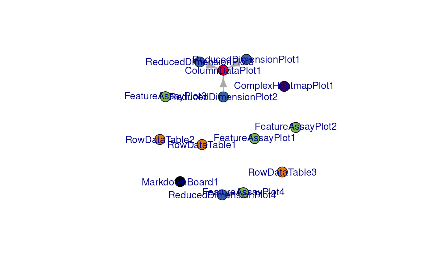

#> IGRAPH 48356ef DN-- 14 4 -- 
#> + attr: name (v/c), color (v/c)
#> + edges from 48356ef (vertex names):
#> [1] ReducedDimensionPlot1->ColumnDataPlot1  
#> [2] ReducedDimensionPlot2->ColumnDataPlot1  
#> [3] ReducedDimensionPlot3->ColumnDataPlot1  
#> [4] ReducedDimensionPlot4->FeatureAssayPlot4

Another alternative for network visualization would use the interactive widget provided by visNetwork:

view_initial_network(initial_1, plot_format = "visNetwork")
#> IGRAPH 8e67e3f DN-- 14 4 -- 
#> + attr: name (v/c), color (v/c)
#> + edges from 8e67e3f (vertex names):
#> [1] ReducedDimensionPlot1->ColumnDataPlot1  
#> [2] ReducedDimensionPlot2->ColumnDataPlot1  
#> [3] ReducedDimensionPlot3->ColumnDataPlot1  
#> [4] ReducedDimensionPlot4->FeatureAssayPlot4

It is also possible to use iSEEfier to combine multiple initial configurations into one:

# create a second initial configuration
feature_list_2 <- c("CD74", "CD79B")
initial_2 <- iSEEinit(sce,
                      features = feature_list_2,
                      clusters = cluster_1)

# merge with the previous one
merged_config <- glue_initials(initial_1, initial_2)
#> Merging together 2 `initial` configuration objects...
#> Combining sets of 14, 10 different panels.
#> 
#> Dropping 1 of the original list of 24 (detected as duplicated entries)
#> 
#> Some names of the panels were specified by the same name, but this situation can be handled at runtime by iSEE
#> (This is just a non-critical message)
#> 
#> Returning an `initial` configuration including 23 different panels. Enjoy!
#> If you want to obtain a preview of the panels configuration, you can call `view_initial_tiles()` on the output of this function

# check out the content of merged_config
view_initial_tiles(initial = merged_config)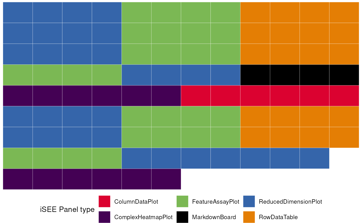

?iSEEfier is always your friend whenever you need further documentation on the package/a certain function and how to use it.

iSEEhub & iSEEindex

iSEEhub: iSEEing the ExperimentHub datasets

The iSEEhub package provides a custom landing page for an iSEE application interfacing with the Bioconductor ExperimentHub. The landing page allows users to browse the ExperimentHub, select a data set, download and cache it, and import it directly into an iSEE app.

library("iSEE")
library("iSEEhub")
#> Loading required package: ExperimentHub
#> Loading required package: AnnotationHub
#> Loading required package: BiocFileCache
#> Loading required package: dbplyr
#> 
#> Attaching package: 'AnnotationHub'
#> The following object is masked from 'package:Biobase':
#> 
#>     cache

ehub <- ExperimentHub()
app <- iSEEhub(ehub)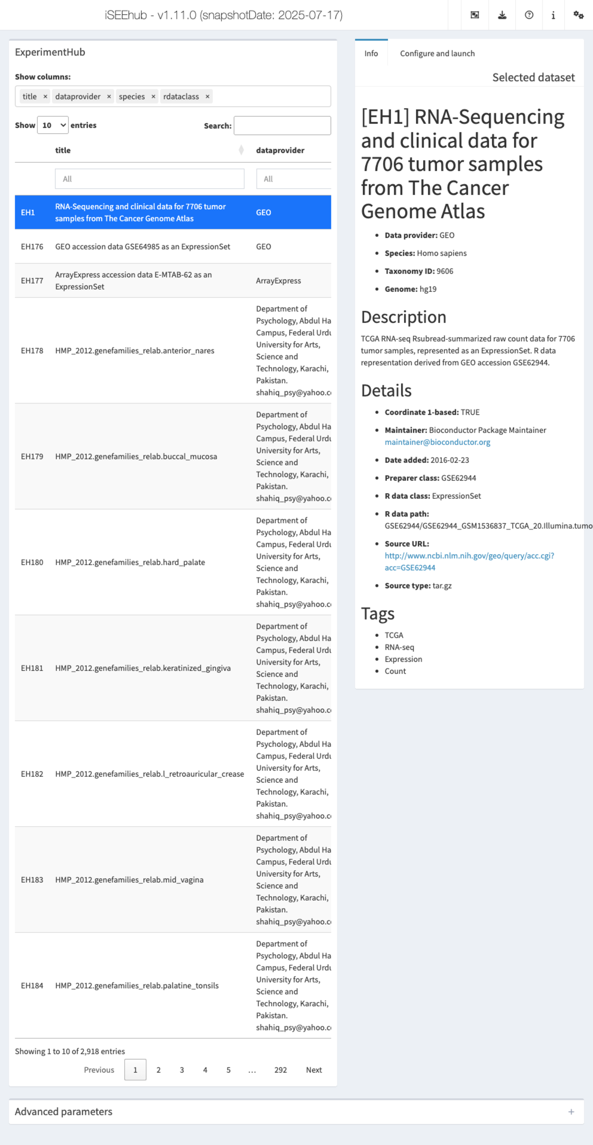

iSEEindex: one instance of iSEE to explore them all

iSEEindex provides an interface to any collection of data sets within a single iSEE web-application.
The main functionality of this package is to define a custom landing page allowing app maintainers to list a custom collection of data sets that users can select from and directly load objects into an iSEE web application. To see how to configure such an app, we will create a small example:

library("iSEE")
library("iSEEindex")

bfc <- BiocFileCache(cache = tempdir())

dataset_fun <- function() {
  x <- yaml::read_yaml(system.file(package = "iSEEindex", "example.yaml"))
  x$datasets
}
initial_fun <- function() {
  x <- yaml::read_yaml(system.file(package = "iSEEindex", "example.yaml"))
  x$initial
}
app <- iSEEindex(bfc, dataset_fun, initial_fun)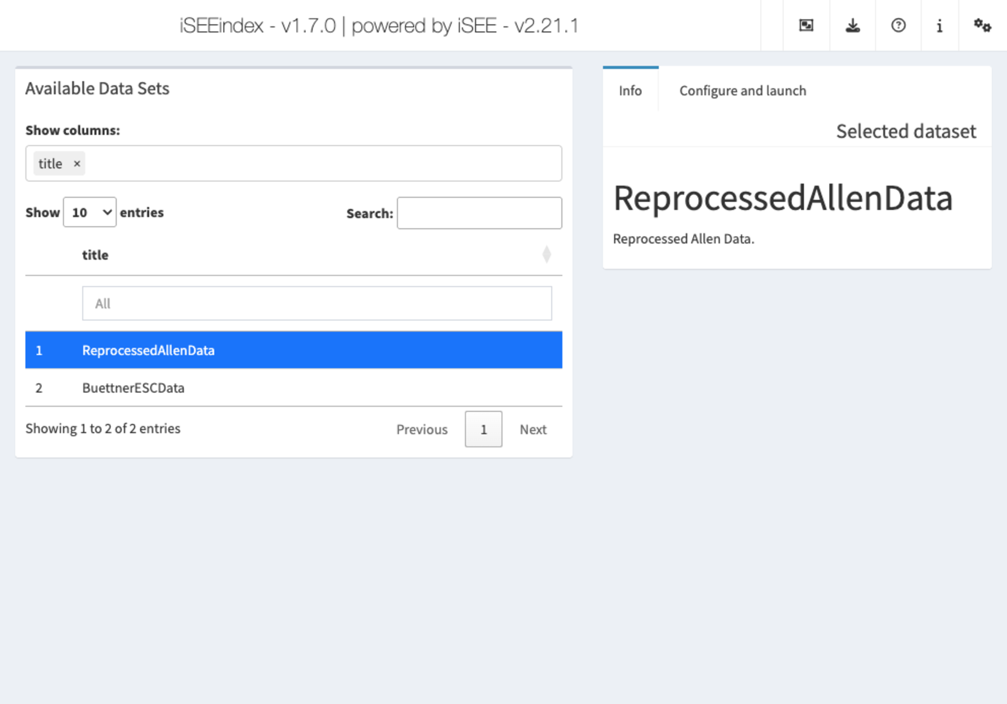

A more elaborate example (referring to the work in (Rigby et al. 2023)) is available at https://rehwinkellab.shinyapps.io/ifnresource/. The source can be found at https://github.com/kevinrue/IFNresource.

Potential use cases can include:

• An app to present and explore the different datasets in your next publication
• An app to explore collection of datasets collaboratively, in consortium-like initiatives
• An app to mirror and enhance the content of e.g. the cellxgene data portal

Tours: help and storytelling

Tours can be an essential tool to satisfy two needs:

• Helping users to navigate the UI
• Telling a story on an existing configuration

A simple example can be demonstrated with this configuration:

sce <- readRDS(
  system.file("datasets", "sce_pbmc3k.RDS", package = "iUSEiSEE")
)

initial_for_tour <- list(
  ReducedDimensionPlot(PanelWidth = 3L), 
  RowDataTable(PanelWidth = 3L),
  FeatureAssayPlot(PanelWidth = 3L),
  ComplexHeatmapPlot(PanelWidth = 3L)
)

This next chunk defines the steps of the tour, specified by an anchoring point (element) and the content of that step (intro).

tour <- data.frame(
  element = c(
    "#Welcome",
    "#ReducedDimensionPlot1",
    "#RowDataTable1",
    "#ComplexHeatmapPlot1",
    "#FeatureAssayPlot1",
    "#ReducedDimensionPlot1",
    "#Conclusion"),
  intro = c(
    "Welcome to this tour!",
    "This is the a reduced dimension plot",
    "and this is a table",
    "Why not a heatmap?",
    "... and now we look at one individual feature.",
    "Back to the a reduced dimension plot...",
    "Thank you for taking this tour!"),
  stringsAsFactors = FALSE
)

app <- iSEE(sce, initial = initial_for_tour, tour = tour)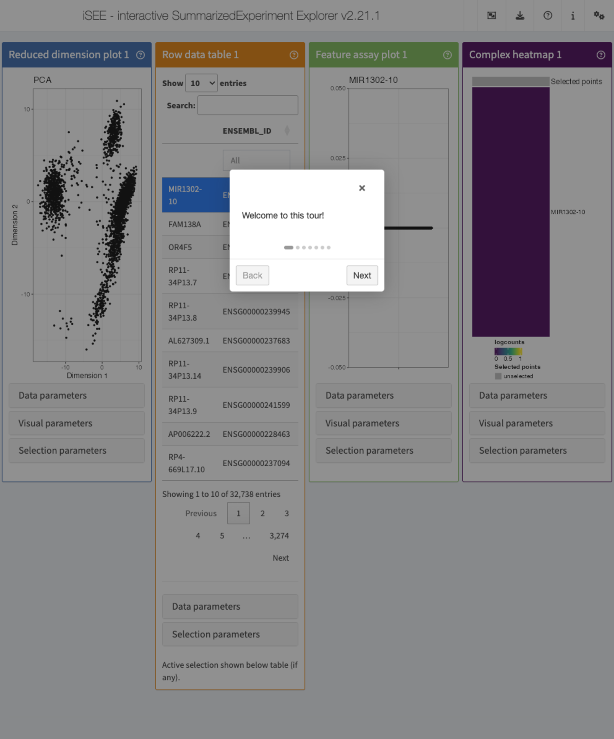

Interoperability

As we have seen throughout this workshop, iSEE works on SummarizedExperiment objects, or derivatives thereof. However, especially if you are working with single-cell data you may already have your dataset available in another format (such as a Seurat object or an AnnData object). To use iSEE on these objects, they first have to be converted to SingleCellExperiment objects. Fortunately, there are good packages available to perform this conversion. We exemplify this below, using data downloaded from https://zenodo.org/records/10084595 (if you want to follow along, download the data and unpack in a folder named datasets in the current working directory).

From Seurat

library("Seurat")

seurat_object <- readRDS("datasets/seurat_pbmc3k.RDS")
sce_from_seurat <- Seurat::as.SingleCellExperiment(
  seurat_object
)
sce_from_seurat

iSEE(sce_from_seurat)

From AnnData

library("zellkonverter")

sce_from_anndata <- zellkonverter::readH5AD(file = "datasets/anndata_pbmc3k.h5ad")
sce_from_anndata

iSEE(sce_from_anndata)

Session info

Session info

sessionInfo()
#> R version 4.5.1 (2025-06-13)
#> Platform: x86_64-pc-linux-gnu
#> Running under: Ubuntu 24.04.2 LTS
#> 
#> Matrix products: default
#> BLAS:   /usr/lib/x86_64-linux-gnu/openblas-pthread/libblas.so.3 
#> LAPACK: /usr/lib/x86_64-linux-gnu/openblas-pthread/libopenblasp-r0.3.26.so;  LAPACK version 3.12.0
#> 
#> locale:
#>  [1] LC_CTYPE=en_US.UTF-8       LC_NUMERIC=C              
#>  [3] LC_TIME=en_US.UTF-8        LC_COLLATE=en_US.UTF-8    
#>  [5] LC_MONETARY=en_US.UTF-8    LC_MESSAGES=en_US.UTF-8   
#>  [7] LC_PAPER=en_US.UTF-8       LC_NAME=C                 
#>  [9] LC_ADDRESS=C               LC_TELEPHONE=C            
#> [11] LC_MEASUREMENT=en_US.UTF-8 LC_IDENTIFICATION=C       
#> 
#> time zone: Etc/UTC
#> tzcode source: system (glibc)
#> 
#> attached base packages:
#> [1] stats4    stats     graphics  grDevices utils     datasets  methods  
#> [8] base     
#> 
#> other attached packages:
#>  [1] iSEEindex_1.6.0             iSEEhub_1.10.0             
#>  [3] ExperimentHub_2.16.1        AnnotationHub_3.16.1       
#>  [5] BiocFileCache_2.16.1        dbplyr_2.5.0               
#>  [7] iSEEfier_1.4.0              GO.db_3.21.0               
#>  [9] org.Hs.eg.db_3.21.0         AnnotationDbi_1.70.0       
#> [11] iSEEpathways_1.6.0          iSEEde_1.6.0               
#> [13] iSEE_2.20.0                 SingleCellExperiment_1.30.1
#> [15] SummarizedExperiment_1.38.1 Biobase_2.68.0             
#> [17] GenomicRanges_1.60.0        GenomeInfoDb_1.44.1        
#> [19] IRanges_2.42.0              S4Vectors_0.46.0           
#> [21] BiocGenerics_0.54.0         generics_0.1.4             
#> [23] MatrixGenerics_1.20.0       matrixStats_1.5.0          
#> [25] BiocStyle_2.36.0           
#> 
#> loaded via a namespace (and not attached):
#>   [1] RColorBrewer_1.1-3      jsonlite_2.0.0          shape_1.4.6.1          
#>   [4] magrittr_2.0.3          farver_2.1.2            rmarkdown_2.29         
#>   [7] GlobalOptions_0.1.2     fs_1.6.6                ragg_1.4.0             
#>  [10] vctrs_0.6.5             memoise_2.0.1           htmltools_0.5.8.1      
#>  [13] S4Arrays_1.8.1          BiocBaseUtils_1.10.0    curl_6.4.0             
#>  [16] SparseArray_1.8.1       sass_0.4.10             bslib_0.9.0            
#>  [19] htmlwidgets_1.6.4       desc_1.4.3              fontawesome_0.5.3      
#>  [22] httr2_1.2.1             listviewer_4.0.0        cachem_1.1.0           
#>  [25] igraph_2.1.4            mime_0.13               lifecycle_1.0.4        
#>  [28] iterators_1.0.14        pkgconfig_2.0.3         colourpicker_1.3.0     
#>  [31] Matrix_1.7-3            R6_2.6.1                fastmap_1.2.0          
#>  [34] GenomeInfoDbData_1.2.14 shiny_1.11.1            clue_0.3-66            
#>  [37] digest_0.6.37           colorspace_2.1-1        paws.storage_0.9.0     
#>  [40] DESeq2_1.48.1           textshaping_1.0.1       RSQLite_2.4.2          
#>  [43] filelock_1.0.3          urltools_1.7.3.1        httr_1.4.7             
#>  [46] abind_1.4-8             mgcv_1.9-3              compiler_4.5.1         
#>  [49] bit64_4.6.0-1           withr_3.0.2             doParallel_1.0.17      
#>  [52] BiocParallel_1.42.1     DBI_1.2.3               shinyAce_0.4.4         
#>  [55] hexbin_1.28.5           rappdirs_0.3.3          DelayedArray_0.34.1    
#>  [58] rjson_0.2.23            tools_4.5.1             vipor_0.4.7            
#>  [61] httpuv_1.6.16           glue_1.8.0              nlme_3.1-168           
#>  [64] promises_1.3.3          grid_4.5.1              cluster_2.1.8.1        
#>  [67] gtable_0.3.6            XVector_0.48.0          stringr_1.5.1          
#>  [70] BiocVersion_3.21.1      ggrepel_0.9.6           foreach_1.5.2          
#>  [73] pillar_1.11.0           limma_3.64.1            later_1.4.2            
#>  [76] rintrojs_0.3.4          circlize_0.4.16         splines_4.5.1          
#>  [79] dplyr_1.1.4             lattice_0.22-7          bit_4.6.0              
#>  [82] paws.common_0.8.5       tidyselect_1.2.1        ComplexHeatmap_2.24.1  
#>  [85] locfit_1.5-9.12         Biostrings_2.76.0       miniUI_0.1.2           
#>  [88] knitr_1.50              edgeR_4.6.3             xfun_0.52              
#>  [91] shinydashboard_0.7.3    statmod_1.5.0           iSEEhex_1.10.0         
#>  [94] DT_0.33                 stringi_1.8.7           visNetwork_2.1.2       
#>  [97] UCSC.utils_1.4.0        yaml_2.3.10             shinyWidgets_0.9.0     
#> [100] evaluate_1.0.4          codetools_0.2-20        tibble_3.3.0           
#> [103] BiocManager_1.30.26     cli_3.6.5               xtable_1.8-4           
#> [106] systemfonts_1.2.3       jquerylib_0.1.4         iSEEu_1.20.0           
#> [109] Rcpp_1.1.0              triebeard_0.4.1         png_0.1-8              
#> [112] parallel_4.5.1          pkgdown_2.1.3           ggplot2_3.5.2          
#> [115] blob_1.2.4              viridisLite_0.4.2       scales_1.4.0           
#> [118] purrr_1.1.0             crayon_1.5.3            GetoptLong_1.0.5       
#> [121] rlang_1.1.6             KEGGREST_1.48.1         shinyjs_2.1.0

References

Alasoo, Kaur, Julia Rodrigues, Subhankar Mukhopadhyay, Andrew J. Knights, Alice L. Mann, Kousik Kundu, Christine Hale, Gordon Dougan, and Daniel J. Gaffney. 2018. “Shared genetic effects on chromatin and gene expression indicate a role for enhancer priming in immune response.” Nature Genetics 50 (3): 424–31. https://doi.org/10.1038/s41588-018-0046-7.

Love, Michael I, Wolfgang Huber, and Simon Anders. 2014. “Moderated estimation of fold change and dispersion for RNA-seq data with DESeq2.” Genome Biology 15 (12): 550. https://doi.org/10.1186/s13059-014-0550-8.

Rigby, Rachel, Kevin Rue-Albrecht, David Sims, and Jan Rehwinkel. 2023. “Single-cell analysis of signalling responses to type I interferons.” bioRxiv, 1–68.