Writing iSEE extensions
Kevin Rue-Albrecht1, Federico Marini2, Charlotte Soneson3
Source:vignettes/workshop_isee_extension.Rmd
workshop_isee_extension.RmdLast modified: 09 July, 2024.
Overview
Description
This package demo will present a brief introduction to the functionality of the iSEE package and its existing extension packages, before demonstrating the writing of new functionality suitable for release in additional extension packages.
Pre-requisites
Workshop prerequisites:
- Familiarity with the SummarizedExperiment class.
- Familiarity with the shiny package
Relevant background reading:
- EuroBioC2023 workshop: materials
- EuroBioC2020 workshop: materials, slides
- BioC2020 workshop: materials, slides
- BioC2019 workshop: materials, slides
- Rue-Albrecht K, Marini F, Soneson C and Lun ATL. iSEE: Interactive SummarizedExperiment Explorer [version 1; peer review: 3 approved]. F1000Research 2018, 7:741 (https://doi.org/10.12688/f1000research.14966.1)
- Vignette: SummarizedExperiment for Coordinating Experimental Assays, Samples, and Regions of Interest
Participation
Students are encouraged to ask questions throughout the package demo.
Where applicable, instructors will illustrate answers with live-coded examples.
Alternatively, students are also encouraged to write questions before, during, and after the workshop using the ‘New issue’ button on the GitHub repository for this workshop (https://github.com/iSEE/iSEEDemoEuroBioC2024/issues).
Instructors will respond to GitHub issues at the earliest opportunity, which may be after the end of the conference.
Time outline
An example for a 40-minute workshop:
| Activity | Time |
|---|---|
| iSEE functionality | 10m |
| Existing iSEE extensions | 10m |
| Writing iSEE extensions | 10m |
| Questions | 10m |
iSEE functionality
Overview
In the next 10 minutes, we will:
- Load a demonstration data set
- Launch an iSEE app in its default state
- Export an R script representing a modified app state
- Re-launch the same iSEE app preconfigured in that modified state
Input data
iSEE was designed around the SummarizedExperiment class, a container widely used throughout the Bioconductor project.
Briefly, the SummarizedExperiment class provides a container keeping matrices of assay data, sample metadata, and feature metadata synchronised throughout analytical workflows (e.g., filtering, reordering).
By extension, iSEE naturally supports classes derived from SummarizedExperiment. For instance, the SingleCellExperiment class adds functionality for storing matrices of reduced dimensions, also keeping those synchronised with assay data and metadata during analyses.
In practice, you would generally create a SummarizedExperiment (or derived) object from raw data and metadata loaded from files (e.g., RNA-seq count matrix produce by a program like featureCounts and sample metadata from your lab notebook).
You can learn about the creation and handling of
SummarizedExperiment objects in the Relevant background reading resources
above.
In this workshop, we will load a publicly available SingleCellExperiment object to save some time.
library(scRNAseq)
sce <- ReprocessedAllenData(assays="tophat_counts")
sce
#> class: SingleCellExperiment
#> dim: 20816 379
#> metadata(2): SuppInfo which_qc
#> assays(1): tophat_counts
#> rownames(20816): 0610007P14Rik 0610009B22Rik ... Zzef1 Zzz3
#> rowData names(0):
#> colnames(379): SRR2140028 SRR2140022 ... SRR2139341 SRR2139336
#> colData names(22): NREADS NALIGNED ... Animal.ID passes_qc_checks_s
#> reducedDimNames(0):
#> mainExpName: endogenous
#> altExpNames(1): ERCC
In the summary view of the object displayed above, we can tell that it contains:
- One assay called
tophat_counts, a matrix measuring 20,816 genes in 379 cells. - Twenty two columns of cell metadata.
- No gene metadata.
Also of note:
- Gene symbols are in use for the row names.
- Arbitrary cell names are in use for column names.
- Some object-level metadata is present.
- An alternative experiment called
ERCCis present (we will not use it).
Getting started with iSEE
One of the strengths of iSEE is that it can be used at any point in an analytical workflow. From the moment raw data or metadata are encapsulated in a SummarizedExperiment object, they’re good to go!
Let’s demonstrate this by attaching the iSEE package
to the R session and calling the iSEE() function to launch
an app in the default settings.
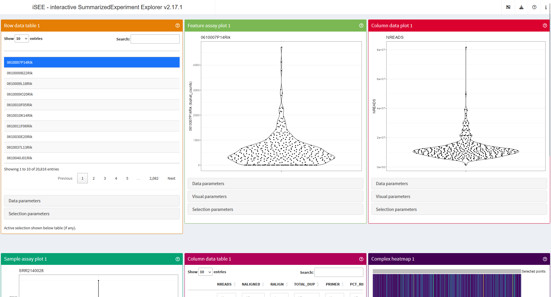
In the screenshot above, you will notice that some of the panels seem to be truncated at the bottom.
iSEE applications organise panels along a single-page layout. Following shiny rules, pages are divided into 12 units horizontally, allowing up to 12 panels on a row before new rows are added to accommodate more panels. Depending on the size and set-up of your monitors, you may comfortably fit a considerable number of panels in your own screen estate.
By default, iSEE applications adopt a “showcase” mode that populates the application with one panel of each type compatible with the assay data and metadata detected in the input object.
As such, in the screenshot above, we see at least:
- A ‘Row data table’ panel, displaying gene metadata.
- A ‘Feature assay plot’ panel, displaying assayed data for a gene.
- A ‘Column data plot’ panel, displaying a column of cell metadata.
- A ‘Sample assay plot’ panel, displaying assayed data for a sample.
- A ‘Column data table’ panel, displaying cell metadata.
- A ‘Complex heatmap’ panel, displaying assayed data for a set of genes.
Core iSEE functionality
Within iSEE applications, users can interactively:
- View tables of metadata, filtering rows, and selecting a single row that may be highlighted in other panels.
- View plots of assay data and metadata, controlling data displayed along each axis, as well as visual aspects such as colour, shape, size, and faceting, using any suitable data or metadata present in the input object.
- Draw selections in plots using the built-in rectangular shiny brush or the slower but more flexible lasso selection implemented in iSEE.
- Transmit selection between panels, dynamically controlling which panels receive information from which panels.
- Use transmitted selections to highlight or restrict the corresponding data points in the receiving panel(s).
- Rearrange the layout of panels, adding, removing, or reordering panels at will.
- Resize the panels, in width and height.
Furthermore, you will also find functionality for:
- Downloading the panel outputs: in PDF format for plots, and CSV format for tables.
- Exporting an R script that reproduces exactly each panel output, including brushes and downstream effects related to transmitted selections.
- Exporting an R script that reproduces exactly the current layout of the application.
- Launching custom interactive tours introducing new users to the various components of the application.
- Opening the vignette of the iSEE package without leaving the application.
- Inspecting the session information.
- Learning more about iSEE, including how to cite it.
- Inspecting the overall object metadata (converted to JSON format).
To simulate a short analytical workflow, let us run some more code
from the ?iSEE help page to:
- Compute a normalised count matrix.
- Compute a PCA.
- Compute a t-SNE.
- Compute some simple gene metadata.
library(scater)
library(scuttle)
sce <- logNormCounts(sce, exprs_values="tophat_counts")

sce <- runPCA(sce, ncomponents=4)
sce <- runTSNE(sce)
rowData(sce)$ave_count <- rowMeans(assay(sce, "tophat_counts"))
rowData(sce)$n_cells <- rowSums(assay(sce, "tophat_counts") > 0)
sce
#> class: SingleCellExperiment
#> dim: 20816 379
#> metadata(2): SuppInfo which_qc
#> assays(2): tophat_counts logcounts
#> rownames(20816): 0610007P14Rik 0610009B22Rik ... Zzef1 Zzz3
#> rowData names(2): ave_count n_cells
#> colnames(379): SRR2140028 SRR2140022 ... SRR2139341 SRR2139336
#> colData names(23): NREADS NALIGNED ... passes_qc_checks_s sizeFactor
#> reducedDimNames(2): PCA TSNE
#> mainExpName: endogenous
#> altExpNames(1): ERCC
Then, as pointed out earlier, you are free to launch another iSEE app again at any point in an analytical workflow.
The iSEE() function automatically detects new assay data
and metadata in the updated object, populating the application
components with all the available information, old and new.
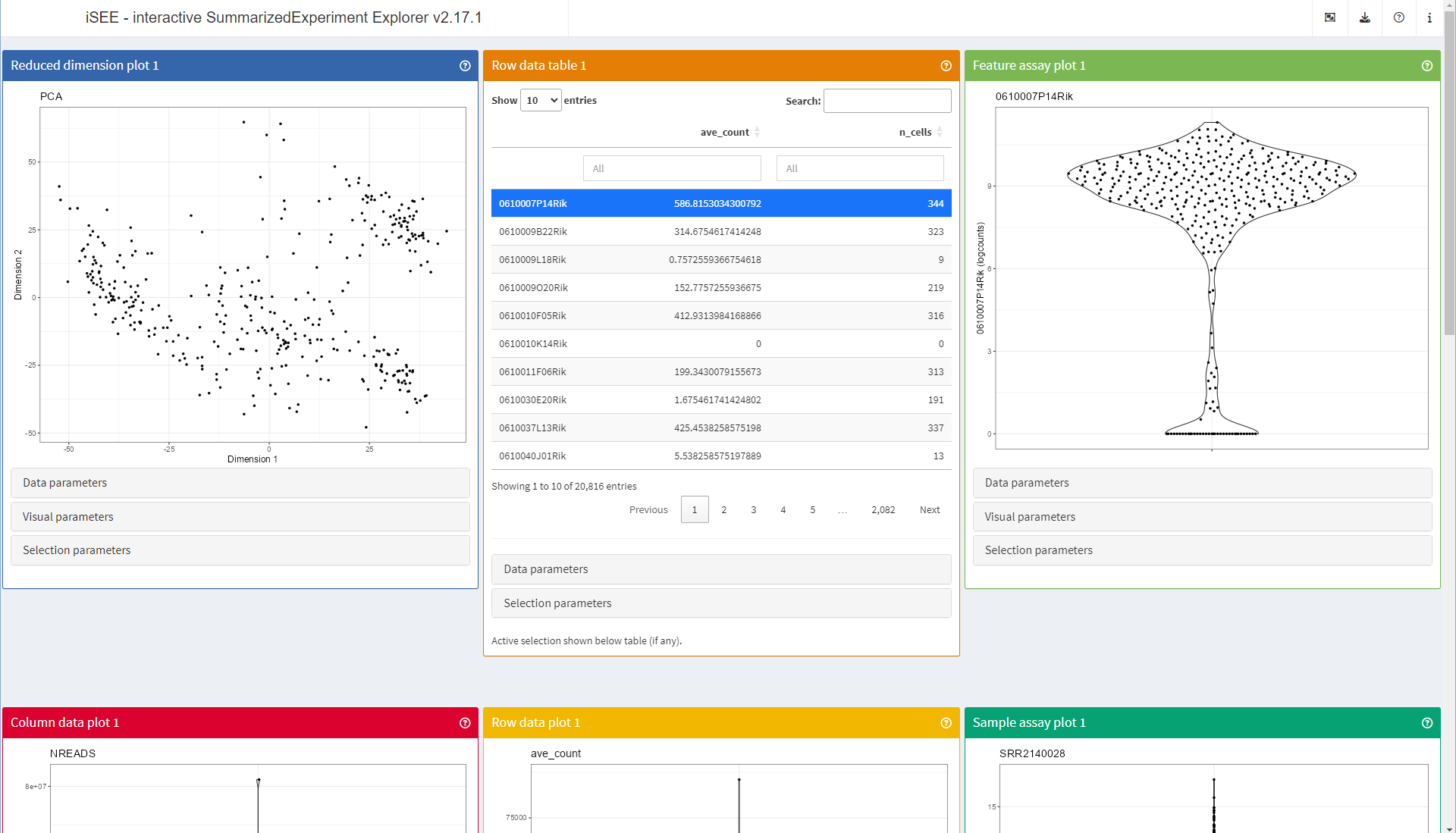
Comparing the screenshot above with the earlier one, you will notice that the first panel is now a ‘Reduced dimension plot’ panel, and that all other panels have shifted position down in the order of the layout (top to bottom, left to right).
Indeed, the last time we launched the app, the object did not contain
any dimensionality reduction result. The iSEE() function
automatically detected that, and dropped that type of panel from the
application.
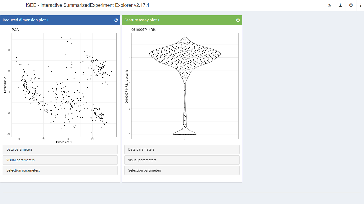
To demonstrate the next functionality, let us interactively (within the app launched above) remove all the panels except for ‘Reduced dimension plot 1’ and ‘Feature assay plot 1’. Then, use the download icon in the navigation bar at the top of the app to find and click the ‘Display panel settings’ button. You will be presented with an R script that looks as follows:
initial <- list()

################################################################################
# Settings for Reduced dimension plot 1
################################################################################

initial[["ReducedDimensionPlot1"]] <- new("ReducedDimensionPlot", Type = "PCA", XAxis = 1L, YAxis = 2L,
    FacetRowByColData = "driver_1_s", FacetColumnByColData = "driver_1_s",
    ColorByColumnData = "NREADS", ColorByFeatureNameAssay = "logcounts",
    ColorBySampleNameColor = "#FF0000", ShapeByColumnData = "driver_1_s",
    SizeByColumnData = "NREADS", TooltipColumnData = character(0),
    FacetRowBy = "None", FacetColumnBy = "None", ColorBy = "None",
    ColorByDefaultColor = "#000000", ColorByFeatureName = "0610007P14Rik",
    ColorByFeatureSource = "---", ColorByFeatureDynamicSource = FALSE,
    ColorBySampleName = "SRR2140028", ColorBySampleSource = "---",
    ColorBySampleDynamicSource = FALSE, ShapeBy = "None", SizeBy = "None",
    SelectionAlpha = 0.1, ZoomData = numeric(0), BrushData = list(),
    VisualBoxOpen = FALSE, VisualChoices = "Color", ContourAdd = FALSE,
    ContourColor = "#0000FF", PointSize = 1, PointAlpha = 1,
    Downsample = FALSE, DownsampleResolution = 200, CustomLabels = FALSE,
    CustomLabelsText = "SRR2140028", FontSize = 1, LegendPointSize = 1,
    LegendPosition = "Bottom", HoverInfo = TRUE, LabelCenters = FALSE,
    LabelCentersBy = "driver_1_s", LabelCentersColor = "#000000",
    VersionInfo = list(iSEE = structure(list(c(2L, 17L, 1L)), class = c("package_version",
    "numeric_version"))), PanelId = c(ReducedDimensionPlot = 1L),
    PanelHeight = 500L, PanelWidth = 4L, SelectionBoxOpen = FALSE,
    RowSelectionSource = "---", ColumnSelectionSource = "---",
    DataBoxOpen = FALSE, RowSelectionDynamicSource = FALSE, ColumnSelectionDynamicSource = FALSE,
    RowSelectionRestrict = FALSE, ColumnSelectionRestrict = FALSE,
    SelectionHistory = list())

################################################################################
# Settings for Feature assay plot 1
################################################################################

initial[["FeatureAssayPlot1"]] <- new("FeatureAssayPlot", Assay = "logcounts", XAxis = "None",
    XAxisColumnData = "NREADS", XAxisFeatureName = "0610007P14Rik",
    XAxisFeatureSource = "---", XAxisFeatureDynamicSource = FALSE,
    YAxisFeatureName = "0610007P14Rik", YAxisFeatureSource = "---",
    YAxisFeatureDynamicSource = FALSE, FacetRowByColData = "driver_1_s",
    FacetColumnByColData = "driver_1_s", ColorByColumnData = "NREADS",
    ColorByFeatureNameAssay = "logcounts", ColorBySampleNameColor = "#FF0000",
    ShapeByColumnData = "driver_1_s", SizeByColumnData = "NREADS",
    TooltipColumnData = character(0), FacetRowBy = "None", FacetColumnBy = "None",
    ColorBy = "None", ColorByDefaultColor = "#000000", ColorByFeatureName = "0610007P14Rik",
    ColorByFeatureSource = "---", ColorByFeatureDynamicSource = FALSE,
    ColorBySampleName = "SRR2140028", ColorBySampleSource = "---",
    ColorBySampleDynamicSource = FALSE, ShapeBy = "None", SizeBy = "None",
    SelectionAlpha = 0.1, ZoomData = numeric(0), BrushData = list(),
    VisualBoxOpen = FALSE, VisualChoices = "Color", ContourAdd = FALSE,
    ContourColor = "#0000FF", PointSize = 1, PointAlpha = 1,
    Downsample = FALSE, DownsampleResolution = 200, CustomLabels = FALSE,
    CustomLabelsText = "SRR2140028", FontSize = 1, LegendPointSize = 1,
    LegendPosition = "Bottom", HoverInfo = TRUE, LabelCenters = FALSE,
    LabelCentersBy = "driver_1_s", LabelCentersColor = "#000000",
    VersionInfo = list(iSEE = structure(list(c(2L, 17L, 1L)), class = c("package_version",
    "numeric_version"))), PanelId = c(FeatureAssayPlot = 1L),
    PanelHeight = 500L, PanelWidth = 4L, SelectionBoxOpen = FALSE,
    RowSelectionSource = "---", ColumnSelectionSource = "---",
    DataBoxOpen = FALSE, RowSelectionDynamicSource = FALSE, ColumnSelectionDynamicSource = FALSE,
    RowSelectionRestrict = FALSE, ColumnSelectionRestrict = FALSE,
    SelectionHistory = list())
The above R script creates an object called initial that
contains all the information necessary for the iSEE()
function to launch an app in a specific initial state.
All we need to do is:
- Run that R script, to create the
initialobject that represents the initial state of the app - Pass this
initialobject to theinitial=argument of theiSEE()function, to launch a new app in the desired initial state
It is useful to note that it is not always necessary to copy-paste R scripts from within the app.
With experience, users can learn to write short scripts from scratch. For instance, the same initial state illustrated above can be achieved using the following script:
initial <- list(
  ReducedDimensionPlot(),
  FeatureAssayPlot()
)
Note that any setting not specified in the R script will be set to a default value that might change in the future. The full R scripts reported by the app ensure complete reproducibility.
Overview
In the next 10 minutes, we will:
- Load and preprocess a new demonstration data set
- Launch an iSEE app that includes panels implemented in extension packages
iSEE extension packages
| Package | Purpose |
|---|---|
| iSEE | Core functionality. |
| iSEEde | Extension for differential expression analysis. |
| iSEEhex | Extension for summarisation into hexagonal bins. |
| iSEEhub | Extension for access to the Bioconductor ExperimentHub. |
| iSEEindex | Extension for access to custom collections of local and remote data sets. |
| iSEEpathways | Extension for pathway analysis. |
| iSEEu | The ‘iSEE universe’: Extension for miscellaneous and experimental functionality. |
In this package demo, we will showcase iSEEde and iSEEpathways.
Input data
Load data
The iSEEpathways
vignette Integration
with other panels can also be accessed locally using the R code
vignette("integration", package = "iSEEpathways").
In this part, we load the airway
package, providing a RangedSummarizedExperiment object for
RNA-Seq in airway smooth muscle cells.
library(airway)
data(airway)
airway
#> class: RangedSummarizedExperiment
#> dim: 63677 8
#> metadata(1): ''
#> assays(1): counts
#> rownames(63677): ENSG00000000003 ENSG00000000005 ... ENSG00000273492
#>   ENSG00000273493
#> rowData names(10): gene_id gene_name ... seq_coord_system symbol
#> colnames(8): SRR1039508 SRR1039509 ... SRR1039520 SRR1039521
#> colData names(9): SampleName cell ... Sample BioSample
Clean up factor levels
We quickly reorder the levels of the dexamethasone treatment, ensuring that the untreated level is first, and used as reference level during the upcoming differential expression analysis.
airway$dex <- relevel(airway$dex, "untrt")Convert gene identifiers to gene symbols
We also take a minute to convert rownames to more recognisable gene symbols using the annotation package org.Hs.eg.db.
To avoid losing any information, we store a copy of the original Ensembl gene identifiers and the corresponding gene symbols in the row metadata.
To make sure that rownames are unique, we use the scuttle
function uniquifyFeatureNames(). The function uses the gene
symbol if unique; otherwise it combines it with the Ensembl gene
identifier to make it unique.
library("org.Hs.eg.db")
library("scuttle")
rowData(airway)[["ENSEMBL"]] <- rownames(airway)
rowData(airway)[["SYMBOL"]] <- mapIds(org.Hs.eg.db, rownames(airway), "SYMBOL", "ENSEMBL")
rowData(airway)[["uniquifyFeatureNames"]] <- uniquifyFeatureNames(
  ID = rowData(airway)[["ENSEMBL"]],
  names = rowData(airway)[["SYMBOL"]]
)
rownames(airway) <- rowData(airway)[["uniquifyFeatureNames"]]
Differential gene expression analysis
We run a standard DESeq2 analysis.
library(DESeq2)
dds <- DESeqDataSet(airway, ~ 0 + dex + cell)
dds <- DESeq(dds)
res_deseq2 <- results(dds, contrast = list("dextrt", "dexuntrt"))
head(res_deseq2)
#> log2 fold change (MLE): dextrt vs dexuntrt
#> Wald test p-value: dextrt vs dexuntrt
#> DataFrame with 6 rows and 6 columns
#>          baseMean log2FoldChange     lfcSE      stat      pvalue       padj
#>         <numeric>      <numeric> <numeric> <numeric>   <numeric>  <numeric>
#> TSPAN6 708.602170     -0.3812539  0.100654 -3.787752 0.000152016 0.00128292
#> TNMD     0.000000             NA        NA        NA          NA         NA
#> DPM1   520.297901      0.2068127  0.112219  1.842944 0.065337213 0.19646961
#> SCYL3  237.163037      0.0379205  0.143445  0.264356 0.791505314 0.91141884
#> FIRRM   57.932633     -0.0881679  0.287142 -0.307054 0.758802543 0.89500551
#> FGR      0.318098     -1.3782416  3.499906 -0.393794 0.693733216         NA
We embed the results of the DESeq2
analysis within the airway object using the iSEEde
function embedContrastResults().
The function embeds the results in a structured way makes them
detectable by the iSEE() function, and gives the
possibility to store multiple differential expression results – possibly
from multiple methods such as edgeR and
limma –
under different names.
library(iSEEde)
airway <- embedContrastResults(res_deseq2, airway, name = "dex: trt vs untrt")
airway
#> class: RangedSummarizedExperiment
#> dim: 63677 8
#> metadata(1): ''
#> assays(1): counts
#> rownames(63677): TSPAN6 TNMD ... APP-DT ENSG00000273493
#> rowData names(14): gene_id gene_name ... uniquifyFeatureNames iSEEde
#> colnames(8): SRR1039508 SRR1039509 ... SRR1039520 SRR1039521
#> colData names(9): SampleName cell ... Sample BioSample
Pathway analysis
We prepare Gene Ontology gene sets of biological pathways using org.Hs.eg.db.
Due to the use of uniquifyFeatureNames() above, we must
first map pathway identifiers to the unique Ensembl gene identifier, to
accurately perform pathway analysis using the feature identifiers
matching those of the embedded differential expression results.
library("org.Hs.eg.db")
pathways <- select(org.Hs.eg.db, head(keys(org.Hs.eg.db, "GOALL"), 100), c("ENSEMBL"), keytype = "GOALL")
pathways <- subset(pathways, ONTOLOGYALL == "BP")
pathways <- unique(pathways[, c("ENSEMBL", "GOALL")])
pathways <- merge(pathways, rowData(airway)[, c("ENSEMBL", "uniquifyFeatureNames")])
pathways <- split(pathways$uniquifyFeatureNames, pathways$GOALL)
We can then run a standard fgsea analysis.
In this case, we rank genes using the log2 fold-change computed
during the differential expression analysis. The iSEEde
function log2FoldChange() is a convenient method to fetch
this information as a named vector in a format immediately compatible
with the fgsea() function. The iSEEde
function contrastResults() is used to fetch embedded
results by name.
library("fgsea")
set.seed(42)
stats <- na.omit(log2FoldChange(contrastResults(airway, "dex: trt vs untrt")))
fgseaRes <- fgsea(pathways = pathways,
                  stats    = stats,
                  minSize  = 15,
                  maxSize  = 500)
#> Warning in preparePathwaysAndStats(pathways, stats, minSize, maxSize, gseaParam, : There are ties in the preranked stats (25.61% of the list).
#> The order of those tied genes will be arbitrary, which may produce unexpected results.
head(fgseaRes[order(pval), ])
#>       pathway       pval      padj   log2err         ES       NES  size
#>        <char>      <num>     <num>     <num>      <num>     <num> <int>
#> 1: GO:0006953 0.08086785 0.6105632 0.2220560  0.4207971  1.344516    36
#> 2: GO:0008585 0.09074074 0.6105632 0.2020717  0.3246918  1.261056    94
#> 3: GO:0022602 0.10074627 0.6105632 0.1918922  0.3846962  1.303461    45
#> 4: GO:0002437 0.16279070 0.6105632 0.1585141 -0.3364185 -1.209283    58
#> 5: GO:0002697 0.19527897 0.6105632 0.1446305 -0.2416966 -1.095904   307
#> 6: GO:0006959 0.19870410 0.6105632 0.1437590 -0.2678407 -1.130609   158
#>     leadingEdge
#>          <list>
#> 1: CD163, S....
#> 2: INHBB, L....
#> 3: LEP, ADA....
#> 4: IL1RN, R....
#> 5: RSAD2, I....
#> 6: TSLP, WF....
Similarly to the differential expression analysis, we embed the
results of the DESeq2
analysis within the airway object, this time using the
iSEEpathways
function embedPathwaysResults().
library("iSEEpathways")
fgseaRes <- fgseaRes[order(pval), ]
airway <- embedPathwaysResults(
  fgseaRes, airway, name = "fgsea (p-value)", class = "fgsea",
  pathwayType = "GO", pathwaysList = pathways, featuresStats = stats)
airway
#> class: RangedSummarizedExperiment
#> dim: 63677 8
#> metadata(2): '' iSEEpathways
#> assays(1): counts
#> rownames(63677): TSPAN6 TNMD ... APP-DT ENSG00000273493
#> rowData names(14): gene_id gene_name ... uniquifyFeatureNames iSEEde
#> colnames(8): SRR1039508 SRR1039509 ... SRR1039520 SRR1039521
#> colData names(9): SampleName cell ... Sample BioSample
Mapping pathways to genes
Separately, it is necessary to define and register a function that fetches the gene identifiers associated with a given pathway identifier. This function is required to transmit selections from pathway-level panels to feature-level panels.
Due to the use of uniquifyFeatureNames() above, the
function must first map to the unique Ensembl gene identifier, to
accurately identify the corresponding value in
rownames(airway).
map_GO <- function(pathway_id, se) {
  pathway_ensembl <- mapIds(org.Hs.eg.db, pathway_id, "ENSEMBL", keytype = "GOALL", multiVals = "CharacterList")[[pathway_id]]
  pathway_rownames <- rownames(se)[rowData(se)[["gene_id"]] %in% pathway_ensembl]
  pathway_rownames
}
airway <- registerAppOptions(airway, Pathways.map.functions = list(GO = map_GO))
Add normalised gene expression
We also compute log-transformed counts, for a better visualisation of differential expression in the live app.
library("scuttle")
airway <- logNormCounts(airway)
Live app
Finally, we can preconfigure the initial state of an app that immediately links panels to one another.
app <- iSEE(airway, initial = list(
  PathwaysTable(PanelWidth = 4L),
  VolcanoPlot(PanelWidth = 4L,
    RowSelectionSource = "PathwaysTable1", ColorBy = "Row selection"),
  ComplexHeatmapPlot(PanelWidth = 4L,
    RowSelectionSource = "PathwaysTable1",
    CustomRows = FALSE, ColumnData = "dex",
    ClusterRows = TRUE, ClusterRowsDistance = "euclidean", AssayCenterRows = TRUE),
  FgseaEnrichmentPlot(PanelWidth = 12L)
))
runApp(app, launch.browser = TRUE)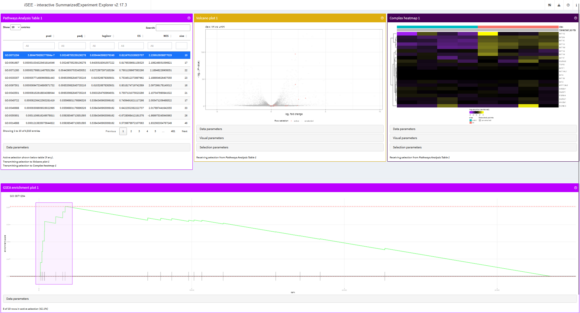
One of the most notable limitations of this app is the delay in
re-rendering panels when users select another pathway. Most of that time
is actually spent in the mapIds() function, querying the
org.Hs.eg.db object. This bottleneck can be circumnavigated
by storing pathways as a regular list() in the
metadata() slot of the airway object, and
changing the mapping function to use that list instead of the
org.Hs.eg.db object, as demonstrated in the section Trading
off memory usage for speed of the iSEEpathways
vignette.
Writing iSEE extensions
Overview
In the next 10 minutes, we will:
- Extend an existing panel class into a new panel class
- Derive a new panel class from an existing panel
Philosophy
iSEE panels are implemented as S4 classes that store the state of each panel in designated slots, and most of the functionality is implemented as S4 methods that describe various behavioural aspects of each panel class.
As a result, new classes can be created simply by inheritance from existing classes, overwriting methods to produce a different behaviour.
Deriving an S4 class
In this demo, let us create a new class called
ReducedDimensionHexPlot, that inherits from the existing
class ReducedDimensionPlot() (implemented in the iSEE
package).
The objective is to produce a panel that displays the same
information as the original ReducedDimensionPlot() panel,
but summarising data points into hexagonal bins.
One major motivation for this functionality is that arbitrarily large data sets comprising many data points may be summarised into a modest number of hexagonal bins, providing a boost in speed when rendering the plot.
However, this is not without caveats:
- Summarising can take many forms (e.g., counting, averaging).
- The ideal number of bins may be different for different data sets.
To proceed, the new class needs at least one additional slot to store the number of hexagonal bins to create (i.e., a resolution for the plot).
setClass("ReducedDimensionHexPlot", contains="ReducedDimensionPlot", slots=c(BinResolution = "numeric"))To properly initialise instances of the new class, the new slot must be populated with a default value in the event that users do not specify a bin resolution.
For this, we need to create a new method for the generic
initialize() and the new class. We set the default
resolution to 100 hexagonal bins along each axis.
Creating a constructor function
It is best practice to give users a function to create objects a particular class. Traditionally, the function is named identically to the class.
In this example, the function passes all its arguments to the
new() function. This is standard practice in iSEE, where
the arguments for constructor functions are typically the values of the
various slots that describe the initial state of the panel.
ReducedDimensionHexPlot <- function(...) {
  new("ReducedDimensionHexPlot", ...)
}
At this point, we can already demonstrate that we have a functional new panel class… that is a carbon copy of the parent class it inherits from!
app <- iSEE(sce, initial = list(
  ReducedDimensionHexPlot(PanelWidth = 6L),
  ReducedDimensionPlot(PanelWidth = 6L)
))
runApp(app, launch.browser = TRUE)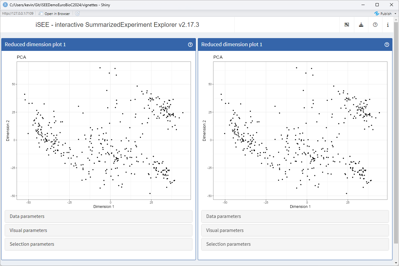
How can we even tell which is which?!
Changing the public panel name
The generic .fullName() declares the label shown in the
interface, at the top of each panel.
Let us create a method for the new class, that gives it a different name, highlighting the hexagonal binning in the plot.
setMethod(".fullName", "ReducedDimensionHexPlot", function(x) "Hexagonal reduced dimension plot")Let’s launch the app to see the effect
app <- iSEE(sce, initial = list(
  ReducedDimensionHexPlot(PanelWidth = 6L),
  ReducedDimensionPlot(PanelWidth = 6L)
))
runApp(app, launch.browser = TRUE)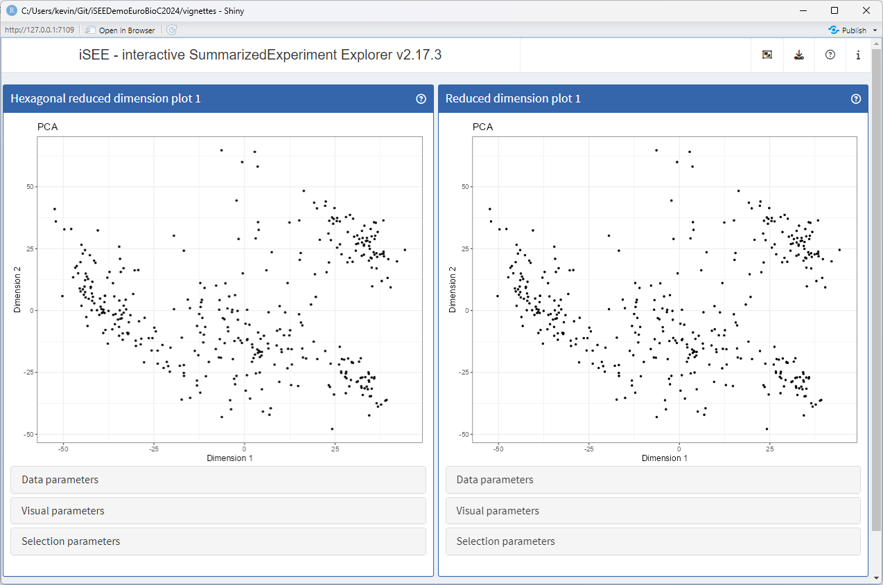
Changing the background panel colour
Similarly, the generic .panelColor() declares the
background colour of the panel header (as well as the colour of brushes
for compatible panels).
Let us create a method for the new class, that gives it a different colour.
setMethod(".panelColor", "ReducedDimensionHexPlot", function(x) "#991717")Let’s launch the app to see the effect
app <- iSEE(sce, initial = list(
  ReducedDimensionHexPlot(PanelWidth = 6L),
  ReducedDimensionPlot(PanelWidth = 6L)
))
runApp(app, launch.browser = TRUE)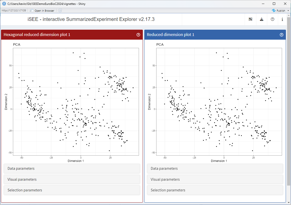
Altering the user interface
At this point, there is still no component in the user interface to control the resolution value store in the new slot.
A number of S4 methods control the interface elements displayed in the various groups of parameters located under each panel.
Here, we are discussing a parameter that will control the size of bins. Moreover, we are about to replace data points by hexagonal bins, meaning that the visual parameters controlling the size of data points are about to become useless.
Thus, the generic .defineVisualSizeInterface() is the
natural choice to use for replacing the size parameters of the parent
ReducedDimensionHexPlot() class by a new HTML element that
displays a numeric input allowing users to change the hexagonal bin
resolution.
setMethod(".defineVisualSizeInterface", "ReducedDimensionHexPlot", function(x) {
  plot_name <- .getEncodedName(x)

  tagList(
    .numericInput.iSEE(x, "BinResolution", label="Bin resolution:",
                       min=1, value=x[["BinResolution"]], step = 1)
  )
})
app <- iSEE(sce, initial = list(
  ReducedDimensionHexPlot(PanelWidth = 6L, VisualBoxOpen = TRUE, VisualChoices = "Size"),
  ReducedDimensionPlot(PanelWidth = 6L, VisualBoxOpen = TRUE, VisualChoices = "Size")
))
runApp(app, launch.browser = TRUE)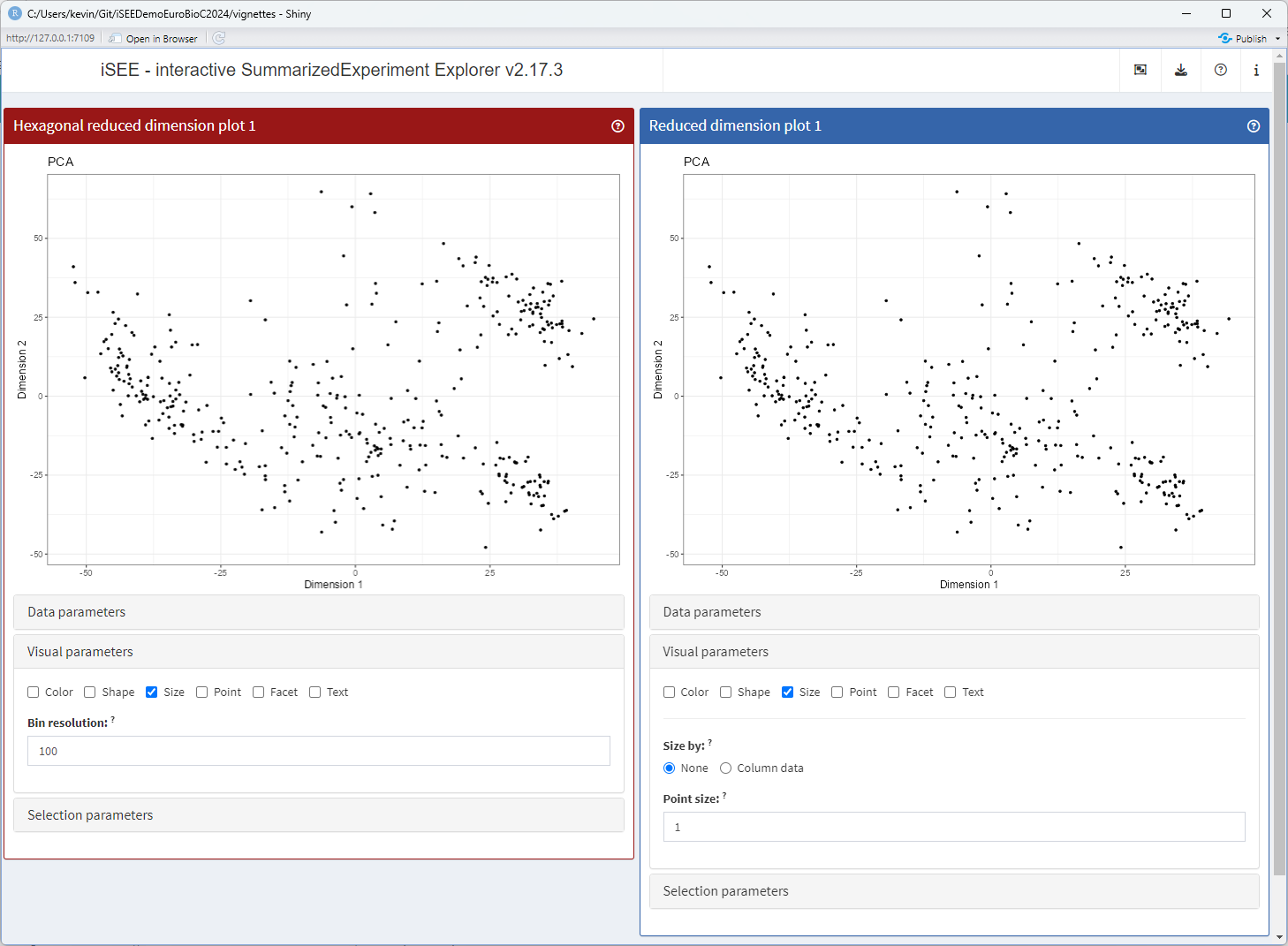
Altering the panel output
Time for the most exciting and challenging task: making the panel produce a different type of plot!
To this end, the generic .generateDotPlot() is key.
Given a panel state, axis labels, and an environment that contains the
SummarizedExperiment() object and possibly other relevant
values such as incoming selections,
setMethod(".generateDotPlot", "ReducedDimensionHexPlot", function(x, labels, envir) {
  plot_cmds <- list()
  plot_cmds[["ggplot"]] <- "ggplot() +"
  color_lab <- "Count"
  new_aes <- .buildAes()
  plot_cmds[["hex"]] <- sprintf(
    "ggplot2::geom_hex(%s, bins = %i, plot.data) +",
    new_aes,
    as.integer(x[["BinResolution"]])
  )
  plot_cmds[["theme_base"]] <- "theme_bw()"

  list(plot=.textEval(plot_cmds, envir), commands=plot_cmds)
})
app <- iSEE(sce, initial = list(
  ReducedDimensionHexPlot(PanelWidth = 6L, VisualBoxOpen = TRUE, VisualChoices = "Size"),
  ReducedDimensionPlot(PanelWidth = 6L, VisualBoxOpen = TRUE, VisualChoices = "Size")
))
runApp(app, launch.browser = TRUE)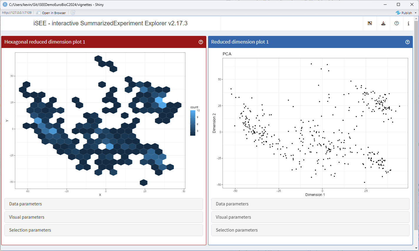
Adding reactivity
At this point, if users change the bin resolution using the newly added interface element, they will notice that nothing seems to happen.
That is because we have not yet added a Shiny observer responding to this particular event.
The .createObservers() generic is invoked to create
observers for all the instances of each panel class added to the user
interface.
The .createProtectedParameterObservers() function
provides a convenient way to create observers responding to events that
change the data being plotted and potentially break active multiple
selections, if any. This function automatically ensures that any change
of value in the interface element is updated in the panel state and
triggers re-rendering of the panel plot.
setMethod(".createObservers", "ReducedDimensionHexPlot", function(x, se, input, session, pObjects, rObjects) {
    callNextMethod()

    plot_name <- .getEncodedName(x)

    .createProtectedParameterObservers(plot_name,
        fields=c("BinResolution"),
        input=input, pObjects=pObjects, rObjects=rObjects)

    invisible(NULL)
})
With the new observer in place, we can launch the app one more time, to toy with the bin resolution and watch the panel plot being re-rendered each time.
app <- iSEE(sce, initial = list(
  ReducedDimensionHexPlot(PanelWidth = 6L, VisualBoxOpen = TRUE, VisualChoices = "Size"),
  ReducedDimensionPlot(PanelWidth = 6L)
))
runApp(app, launch.browser = TRUE)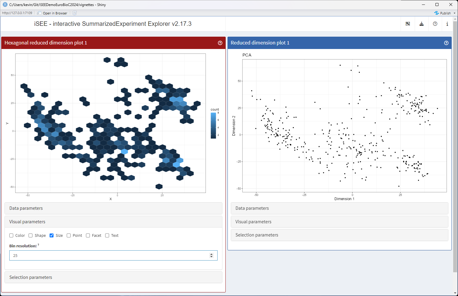
Further work
At this point, there are many more aspects of the plotting behaviour that we should test and adjust, making sure that all the choices of parameters presented to end users are sensible, and that all combinations of parameters are handled without error.
However, that work represents many hours of careful testing and implementation that is far beyond the scope of this short package demo.
Adventurous souls may be interested in a more mature implementation
of the ReducedDimensionHexPlot() panel class, implemented
in the iSEEhex
package. Source code can be found on GitHub on this
page.
Additional resources
The book Extending iSEE is the original effort from developers to provide guidance for writing iSEE extensions using example use cases for illustration.
The more recent iSEETheBook launched a new effort to provide a comprehensive view of the ecosystem for all three major groups of users:
- End users interacting with the graphical user interface in their web browser.
- Developers of scripted web-applications using iSEE to showcase data sets.
- Developers of extensions contributing new functionality and packages to the iSEE ecosystem.
The iSEE website is the place to watch for links to additional resources.
Session info
sessioninfo::session_info()
#> ─ Session info ───────────────────────────────────────────────────────────────
#>  setting  value
#>  version  R version 4.4.1 (2024-06-14)
#>  os       Ubuntu 22.04.4 LTS
#>  system   x86_64, linux-gnu
#>  ui       X11
#>  language en
#>  collate  en_US.UTF-8
#>  ctype    en_US.UTF-8
#>  tz       Etc/UTC
#>  date     2024-09-05
#>  pandoc   3.3 @ /usr/bin/ (via rmarkdown)
#>
#> ─ Packages ───────────────────────────────────────────────────────────────────
#>  package              * version   date (UTC) lib source
#>  abind                  1.4-5     2016-07-21 [2] RSPM (R 4.4.0)
#>  airway               * 1.25.0    2024-05-02 [2] Bioconductor 3.20 (R 4.4.0)
#>  alabaster.base         1.5.6     2024-08-28 [2] Bioconductor 3.20 (R 4.4.1)
#>  alabaster.matrix       1.5.5     2024-07-21 [2] Bioconductor 3.20 (R 4.4.1)
#>  alabaster.ranges       1.5.2     2024-06-23 [2] Bioconductor 3.20 (R 4.4.1)
#>  alabaster.sce          1.5.1     2024-05-24 [2] Bioconductor 3.20 (R 4.4.0)
#>  alabaster.schemas      1.5.0     2024-05-01 [2] Bioconductor 3.20 (R 4.4.0)
#>  alabaster.se           1.5.3     2024-07-05 [2] Bioconductor 3.20 (R 4.4.1)
#>  AnnotationDbi        * 1.67.0    2024-05-01 [2] Bioconductor 3.20 (R 4.4.0)
#>  AnnotationFilter       1.29.0    2024-05-01 [2] Bioconductor 3.20 (R 4.4.0)
#>  AnnotationHub          3.13.3    2024-08-19 [2] Bioconductor 3.20 (R 4.4.1)
#>  beachmat               2.21.5    2024-07-26 [2] Bioconductor 3.20 (R 4.4.1)
#>  beeswarm               0.4.0     2021-06-01 [2] RSPM (R 4.4.0)
#>  Biobase              * 2.65.1    2024-08-28 [2] Bioconductor 3.20 (R 4.4.1)
#>  BiocFileCache          2.13.0    2024-05-01 [2] Bioconductor 3.20 (R 4.4.0)
#>  BiocGenerics         * 0.51.1    2024-09-03 [2] Bioconductor 3.20 (R 4.4.1)
#>  BiocIO                 1.15.2    2024-08-23 [2] Bioconductor 3.20 (R 4.4.1)
#>  BiocManager            1.30.25   2024-08-28 [2] CRAN (R 4.4.1)
#>  BiocNeighbors          1.23.0    2024-05-01 [2] Bioconductor 3.20 (R 4.4.0)
#>  BiocParallel           1.39.0    2024-05-01 [2] Bioconductor 3.20 (R 4.4.0)
#>  BiocSingular           1.21.2    2024-07-04 [2] Bioconductor 3.20 (R 4.4.1)
#>  BiocStyle              2.33.1    2024-06-12 [2] Bioconductor 3.20 (R 4.4.0)
#>  BiocVersion            3.20.0    2024-05-01 [2] Bioconductor 3.20 (R 4.4.1)
#>  Biostrings             2.73.1    2024-06-02 [2] Bioconductor 3.20 (R 4.4.0)
#>  bit                    4.0.5     2022-11-15 [2] RSPM (R 4.4.0)
#>  bit64                  4.0.5     2020-08-30 [2] RSPM (R 4.4.0)
#>  bitops                 1.0-8     2024-07-29 [2] RSPM (R 4.4.0)
#>  blob                   1.2.4     2023-03-17 [2] RSPM (R 4.4.0)
#>  bslib                  0.8.0     2024-07-29 [2] RSPM (R 4.4.0)
#>  cachem                 1.1.0     2024-05-16 [2] RSPM (R 4.4.0)
#>  circlize               0.4.16    2024-02-20 [2] RSPM (R 4.4.0)
#>  cli                    3.6.3     2024-06-21 [2] RSPM (R 4.4.0)
#>  clue                   0.3-65    2023-09-23 [2] RSPM (R 4.4.0)
#>  cluster                2.1.6     2023-12-01 [3] CRAN (R 4.4.1)
#>  codetools              0.2-20    2024-03-31 [3] CRAN (R 4.4.1)
#>  colorspace             2.1-1     2024-07-26 [2] RSPM (R 4.4.0)
#>  colourpicker           1.3.0     2023-08-21 [2] RSPM (R 4.4.0)
#>  ComplexHeatmap         2.21.0    2024-05-01 [2] Bioconductor 3.20 (R 4.4.0)
#>  cowplot                1.1.3     2024-01-22 [2] RSPM (R 4.4.0)
#>  crayon                 1.5.3     2024-06-20 [2] RSPM (R 4.4.0)
#>  curl                   5.2.2     2024-08-26 [2] RSPM (R 4.4.0)
#>  data.table             1.16.0    2024-08-27 [2] RSPM (R 4.4.0)
#>  DBI                    1.2.3     2024-06-02 [2] RSPM (R 4.4.0)
#>  dbplyr                 2.5.0     2024-03-19 [2] RSPM (R 4.4.0)
#>  DelayedArray           0.31.11   2024-08-04 [2] Bioconductor 3.20 (R 4.4.1)
#>  desc                   1.4.3     2023-12-10 [2] RSPM (R 4.4.0)
#>  DESeq2               * 1.45.3    2024-07-24 [2] Bioconductor 3.20 (R 4.4.1)
#>  digest                 0.6.37    2024-08-19 [2] RSPM (R 4.4.0)
#>  doParallel             1.0.17    2022-02-07 [2] RSPM (R 4.4.0)
#>  dplyr                  1.1.4     2023-11-17 [2] RSPM (R 4.4.0)
#>  DT                     0.33      2024-04-04 [2] RSPM (R 4.4.0)
#>  edgeR                  4.3.14    2024-09-01 [2] Bioconductor 3.20 (R 4.4.1)
#>  ensembldb              2.29.1    2024-08-21 [2] Bioconductor 3.20 (R 4.4.1)
#>  evaluate               0.24.0    2024-06-10 [2] RSPM (R 4.4.0)
#>  ExperimentHub          2.13.1    2024-07-31 [2] Bioconductor 3.20 (R 4.4.1)
#>  fansi                  1.0.6     2023-12-08 [2] RSPM (R 4.4.0)
#>  fastmap                1.2.0     2024-05-15 [2] RSPM (R 4.4.0)
#>  fastmatch              1.1-4     2023-08-18 [2] RSPM (R 4.4.0)
#>  fgsea                * 1.31.0    2024-05-01 [2] Bioconductor 3.20 (R 4.4.0)
#>  filelock               1.0.3     2023-12-11 [2] RSPM (R 4.4.0)
#>  fontawesome            0.5.2     2023-08-19 [2] RSPM (R 4.4.0)
#>  foreach                1.5.2     2022-02-02 [2] RSPM (R 4.4.0)
#>  fs                     1.6.4     2024-04-25 [2] RSPM (R 4.4.0)
#>  generics               0.1.3     2022-07-05 [2] RSPM (R 4.4.0)
#>  GenomeInfoDb         * 1.41.1    2024-05-24 [2] Bioconductor 3.20 (R 4.4.0)
#>  GenomeInfoDbData       1.2.12    2024-06-24 [2] Bioconductor
#>  GenomicAlignments      1.41.0    2024-05-01 [2] Bioconductor 3.20 (R 4.4.0)
#>  GenomicFeatures        1.57.0    2024-05-01 [2] Bioconductor 3.20 (R 4.4.0)
#>  GenomicRanges        * 1.57.1    2024-06-12 [2] Bioconductor 3.20 (R 4.4.0)
#>  GetoptLong             1.0.5     2020-12-15 [2] RSPM (R 4.4.0)
#>  ggbeeswarm             0.7.2     2023-04-29 [2] RSPM (R 4.4.0)
#>  ggplot2              * 3.5.1     2024-04-23 [2] RSPM (R 4.4.0)
#>  ggrepel                0.9.5     2024-01-10 [2] RSPM (R 4.4.0)
#>  GlobalOptions          0.1.2     2020-06-10 [2] RSPM (R 4.4.0)
#>  glue                   1.7.0     2024-01-09 [2] RSPM (R 4.4.0)
#>  gridExtra              2.3       2017-09-09 [2] RSPM (R 4.4.0)
#>  gtable                 0.3.5     2024-04-22 [2] RSPM (R 4.4.0)
#>  gypsum                 1.1.6     2024-06-23 [2] Bioconductor 3.20 (R 4.4.1)
#>  HDF5Array              1.33.6    2024-08-11 [2] Bioconductor 3.20 (R 4.4.1)
#>  htmltools              0.5.8.1   2024-04-04 [2] RSPM (R 4.4.0)
#>  htmlwidgets            1.6.4     2023-12-06 [2] RSPM (R 4.4.0)
#>  httpuv                 1.6.15    2024-03-26 [2] RSPM (R 4.4.0)
#>  httr                   1.4.7     2023-08-15 [2] RSPM (R 4.4.0)
#>  httr2                  1.0.3     2024-08-22 [2] RSPM (R 4.4.0)
#>  igraph                 2.0.3     2024-03-13 [2] RSPM (R 4.4.0)
#>  IRanges              * 2.39.2    2024-07-17 [2] Bioconductor 3.20 (R 4.4.1)
#>  irlba                  2.3.5.1   2022-10-03 [2] RSPM (R 4.4.0)
#>  iSEE                 * 2.17.4    2024-09-03 [2] Bioconductor 3.20 (R 4.4.1)
#>  iSEEde               * 1.3.0     2024-05-01 [2] Bioconductor 3.20 (R 4.4.0)
#>  iSEEpathways         * 1.3.0     2024-05-01 [2] Bioconductor 3.20 (R 4.4.0)
#>  iterators              1.0.14    2022-02-05 [2] RSPM (R 4.4.0)
#>  jquerylib              0.1.4     2021-04-26 [2] RSPM (R 4.4.0)
#>  jsonlite               1.8.8     2023-12-04 [2] RSPM (R 4.4.0)
#>  KEGGREST               1.45.1    2024-06-17 [2] Bioconductor 3.20 (R 4.4.0)
#>  knitr                  1.48      2024-07-07 [2] RSPM (R 4.4.0)
#>  later                  1.3.2     2023-12-06 [2] RSPM (R 4.4.0)
#>  lattice                0.22-6    2024-03-20 [3] CRAN (R 4.4.1)
#>  lazyeval               0.2.2     2019-03-15 [2] RSPM (R 4.4.0)
#>  lifecycle              1.0.4     2023-11-07 [2] RSPM (R 4.4.0)
#>  limma                  3.61.9    2024-08-04 [2] Bioconductor 3.20 (R 4.4.1)
#>  listviewer             4.0.0     2023-09-30 [2] RSPM (R 4.4.0)
#>  locfit                 1.5-9.10  2024-06-24 [2] RSPM (R 4.4.0)
#>  magrittr               2.0.3     2022-03-30 [2] RSPM (R 4.4.0)
#>  Matrix                 1.7-0     2024-04-26 [3] CRAN (R 4.4.1)
#>  MatrixGenerics       * 1.17.0    2024-05-01 [2] Bioconductor 3.20 (R 4.4.0)
#>  matrixStats          * 1.4.0     2024-09-04 [2] RSPM (R 4.4.0)
#>  memoise                2.0.1     2021-11-26 [2] RSPM (R 4.4.0)
#>  mgcv                   1.9-1     2023-12-21 [3] CRAN (R 4.4.1)
#>  mime                   0.12      2021-09-28 [2] RSPM (R 4.4.0)
#>  miniUI                 0.1.1.1   2018-05-18 [2] RSPM (R 4.4.0)
#>  munsell                0.5.1     2024-04-01 [2] RSPM (R 4.4.0)
#>  nlme                   3.1-166   2024-08-14 [2] RSPM (R 4.4.0)
#>  org.Hs.eg.db         * 3.19.1    2024-06-24 [2] Bioconductor
#>  pillar                 1.9.0     2023-03-22 [2] RSPM (R 4.4.0)
#>  pkgconfig              2.0.3     2019-09-22 [2] RSPM (R 4.4.0)
#>  pkgdown                2.1.0     2024-07-06 [2] RSPM (R 4.4.0)
#>  png                    0.1-8     2022-11-29 [2] RSPM (R 4.4.0)
#>  promises               1.3.0     2024-04-05 [2] RSPM (R 4.4.0)
#>  ProtGenerics           1.37.1    2024-07-31 [2] Bioconductor 3.20 (R 4.4.1)
#>  R6                     2.5.1     2021-08-19 [2] RSPM (R 4.4.0)
#>  ragg                   1.3.2     2024-05-15 [2] RSPM (R 4.4.0)
#>  rappdirs               0.3.3     2021-01-31 [2] RSPM (R 4.4.0)
#>  RColorBrewer           1.1-3     2022-04-03 [2] RSPM (R 4.4.0)
#>  Rcpp                   1.0.13    2024-07-17 [2] RSPM (R 4.4.0)
#>  RCurl                  1.98-1.16 2024-07-11 [2] RSPM (R 4.4.0)
#>  restfulr               0.0.15    2022-06-16 [2] RSPM (R 4.4.0)
#>  rhdf5                  2.49.0    2024-05-01 [2] Bioconductor 3.20 (R 4.4.0)
#>  rhdf5filters           1.17.0    2024-05-01 [2] Bioconductor 3.20 (R 4.4.0)
#>  Rhdf5lib               1.27.0    2024-05-01 [2] Bioconductor 3.20 (R 4.4.0)
#>  rintrojs               0.3.4     2024-01-11 [2] RSPM (R 4.4.0)
#>  rjson                  0.2.22    2024-08-20 [2] RSPM (R 4.4.0)
#>  rlang                  1.1.4     2024-06-04 [2] RSPM (R 4.4.0)
#>  rmarkdown              2.28      2024-08-17 [2] RSPM (R 4.4.0)
#>  Rsamtools              2.21.1    2024-08-16 [2] Bioconductor 3.20 (R 4.4.1)
#>  RSQLite                2.3.7     2024-05-27 [2] RSPM (R 4.4.0)
#>  rsvd                   1.0.5     2021-04-16 [2] RSPM (R 4.4.0)
#>  rtracklayer            1.65.0    2024-05-01 [2] Bioconductor 3.20 (R 4.4.0)
#>  Rtsne                  0.17      2023-12-07 [2] RSPM (R 4.4.0)
#>  S4Arrays               1.5.7     2024-08-06 [2] Bioconductor 3.20 (R 4.4.1)
#>  S4Vectors            * 0.43.2    2024-07-17 [2] Bioconductor 3.20 (R 4.4.1)
#>  sass                   0.4.9     2024-03-15 [2] RSPM (R 4.4.0)
#>  ScaledMatrix           1.13.0    2024-05-01 [2] Bioconductor 3.20 (R 4.4.0)
#>  scales                 1.3.0     2023-11-28 [2] RSPM (R 4.4.0)
#>  scater               * 1.33.4    2024-07-21 [2] Bioconductor 3.20 (R 4.4.1)
#>  scRNAseq             * 2.19.1    2024-06-25 [2] Bioconductor 3.20 (R 4.4.1)
#>  scuttle              * 1.15.4    2024-08-14 [2] Bioconductor 3.20 (R 4.4.1)
#>  sessioninfo            1.2.2     2021-12-06 [2] RSPM (R 4.4.0)
#>  shape                  1.4.6.1   2024-02-23 [2] RSPM (R 4.4.0)
#>  shiny                  1.9.1     2024-08-01 [2] RSPM (R 4.4.0)
#>  shinyAce               0.4.2     2022-05-06 [2] RSPM (R 4.4.0)
#>  shinydashboard         0.7.2     2021-09-30 [2] RSPM (R 4.4.0)
#>  shinyjs                2.1.0     2021-12-23 [2] RSPM (R 4.4.0)
#>  shinyWidgets           0.8.6     2024-04-24 [2] RSPM (R 4.4.0)
#>  SingleCellExperiment * 1.27.2    2024-05-24 [2] Bioconductor 3.20 (R 4.4.0)
#>  SparseArray            1.5.31    2024-08-04 [2] Bioconductor 3.20 (R 4.4.1)
#>  statmod                1.5.0     2023-01-06 [2] RSPM (R 4.4.0)
#>  SummarizedExperiment * 1.35.1    2024-06-28 [2] Bioconductor 3.20 (R 4.4.1)
#>  systemfonts            1.1.0     2024-05-15 [2] RSPM (R 4.4.0)
#>  textshaping            0.4.0     2024-05-24 [2] RSPM (R 4.4.0)
#>  tibble                 3.2.1     2023-03-20 [2] RSPM (R 4.4.0)
#>  tidyselect             1.2.1     2024-03-11 [2] RSPM (R 4.4.0)
#>  UCSC.utils             1.1.0     2024-05-01 [2] Bioconductor 3.20 (R 4.4.0)
#>  utf8                   1.2.4     2023-10-22 [2] RSPM (R 4.4.0)
#>  vctrs                  0.6.5     2023-12-01 [2] RSPM (R 4.4.0)
#>  vipor                  0.4.7     2023-12-18 [2] RSPM (R 4.4.0)
#>  viridis                0.6.5     2024-01-29 [2] RSPM (R 4.4.0)
#>  viridisLite            0.4.2     2023-05-02 [2] RSPM (R 4.4.0)
#>  withr                  3.0.1     2024-07-31 [2] RSPM (R 4.4.0)
#>  xfun                   0.47      2024-08-17 [2] RSPM (R 4.4.0)
#>  XML                    3.99-0.17 2024-06-25 [2] RSPM (R 4.4.0)
#>  xtable                 1.8-4     2019-04-21 [2] RSPM (R 4.4.0)
#>  XVector                0.45.0    2024-05-01 [2] Bioconductor 3.20 (R 4.4.0)
#>  yaml                   2.3.10    2024-07-26 [2] RSPM (R 4.4.0)
#>  zlibbioc               1.51.1    2024-06-05 [2] Bioconductor 3.20 (R 4.4.0)
#>
#>  [1] /tmp/RtmpzEmLBL/temp_libpath1af82484df26
#>  [2] /usr/local/lib/R/site-library
#>  [3] /usr/local/lib/R/library
#>
#> ──────────────────────────────────────────────────────────────────────────────